The ARRAYFORMULA function in Google Sheets is useful to apply a formula to an entire column in Google Sheets. In other words, it converts a formula that returns one value into a formula that returns an array.
Table of Contents
The use of ARRAYFORMULAs sounds scary and difficult to understand at first. To see what their purpose is, let me explain what an ARRAYFORMULA is.
When working with a large data set, it is common to repeat similar formulas across the length of a column. When using a regular formula (without ARRAYFORMULA), you can put a formula in the first line of the data set:
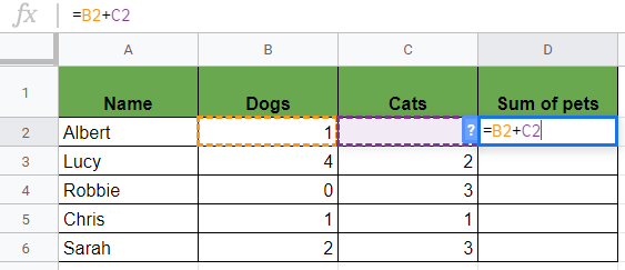
And then drag down the formula in the next rows:

Google Sheets will automatically adjust the formula of the first cell in the following rows, and it will apply the same calculations with the respective row numbers until the row where you dragged it down. Therefore, the calculation =B2+C2 in the second line will be changed to =B3+C3 automatically in the third row, and so on.
It is a pretty easy way to apply a structurally similar formula to a list of data, and in many simple cases, it is enough to do it like this.
However, you can automate this process completely using an ARRAYFORMULA which allows you more flexibility and dynamics with the data when working in batch.
As its name suggests, the ARRAYFORMULA function applies a formula to a whole array (we call ranges of connected values arrays). You only need to enter the formula in a single cell and wrap it into an ARRAYFORMULA. It expands automatically to all the rows down in the range.
The Anatomy of the ARRAYFORMULA Function
The syntax of ARRAYFORMULA isn’t too self-explanatory, but you will see examples of how to use it below. So the syntax (the way we write it) is:
=ARRAYFORMULA(array_formula)
Let’s break it down and understand what each of the components mean:
=the equal sign is just how we start any function in Google Sheets.ARRAYFORMULA()is our function. When using theARRAYFORMULAfunction We will have to provide the correspondingarray_formulaattribute for it to work.array_formulais the formula we want to apply to the whole array. By definition, it can either be a range, a mathematical expression using one cell range or multiple ranges of the same size. Additionally, it can also be a function that returns a result greater than one cell.
The difference from the drag-down copy and paste solution is that here all you need to change is the single cell references in your formula into references that refer to a column or range of cells. As aforementioned above, this will automate the entire process and make it quicker.
How to Use ARRAYFORMULA with a Mathematical Expression
Say you would like to add the values of column B and C from the first to the tenth row and instead of doing it one by one, you use an ARRAYFORMULA. You should add the two ranges of the same size, and as a result, it will return an array of the same size that contains the summarized values of each row from 1 to 10.
=ARRAYFORMULA(B1:B10 + C1:C10)
This formula has an ARRAYFORMULA with a mathematical expression (addition) inside. You can create similar formulas using subtraction, multiplication, raising to powers, etc. and all the variety of their combinations.
Furthermore, the syntax of the ARRAYFORMULA function defines that apart from mathematical expressions, you can also use single ranges or functions as well.
How to Use ARRAYFORMULA with a Single Range
When you want to use single ranges in an ARRAYFORMULA:
- You can put a single range into an array formula as well. It will copy the values from the selected column to your array. You can write the following expression to copy the content of column A starting from A1:
=ARRAYFORMULA(A1:A)
- You can do the same horizontally as well when using an
ARRAYFORMULAthrough a row. This expression will copy the content of the first row starting from A1:=ARRAYFORMULA(A1:1)
How to Use ARRAYFORMULA with a Function
The most powerful and seemingly most complicated option is to wrap another function in an ARRAYFORMULA. It enables you to use arrays in non-array functions. You can create repetitive calculations across a whole data range while writing the function only in the first cell of the array.
There are endless opportunities with ARRAYFORMULA for beginner and advanced users as well, and it can make your sheets a lot more automated and flexible.
=ARRAYFORMULA(function())
The function() inside can be any function that is applied to the whole array.
You can see a step-by-step guide in the last section (“How to Use ARRAYFORMULA Function in Google Sheets”) down below this post where we use ARRAYFORMULA with an IF expression inside.
⚠️ Notes to Use ARRAYFORMULA Function Perfectly
- Each array has to be of the same size to operate between arrays.
- Pressing Ctrl+Shift+Enter while editing a formula will automatically add
ARRAYFORMULA(to the beginning of the formula. - You can make changes in just one cell, and the effect takes place across the data range of the
ARRAYFORMULA. - Advanced users can combine the
ARRAYFORMULAwith a lot of other functions, but it does not work withFILTERorQUERY.
A Real Example of Using ARRAYFORMULA Function
Let’s see how to use ARRAYFORMULA function in Google Sheets with the previous example of the number of pets. We want to apply the same addition formula as before which is a mathematical expression. But instead of doing in it every single cell, we wrap it in an ARRAYFORMULA.
Therefore we have to change the single cell references into range references in the following way to apply the addition to the whole column.
=ARRAYFORMULA(B2:B + C2:C)
We put this formula in the cell E2:

If a single cell reference was B2 before, now we change it into the whole column starting from B2, so we write B2:B. After hitting Enter, Google Sheets will automatically apply the same calculation to the entire array.
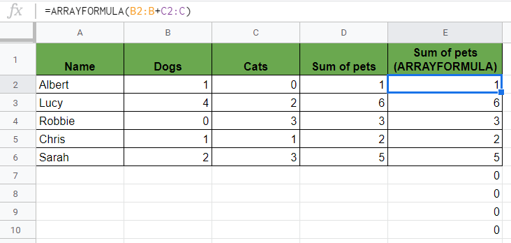
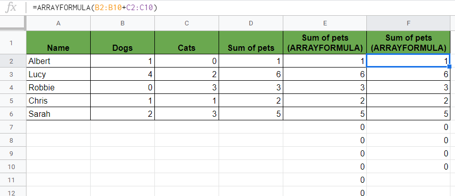
You can see that the ARRAYFORMULA is applied to the whole column, and there is an infinite number of zeros at the end. If you don’t want these infinite columns, you can set a limit to your range in the ARRAYFORMULA as well, so, for example, instead of applying it to the whole column (B2:B+C2:C), only apply it until the 10th row with the formula below:
=ARRAYFORMULA(B2:B10 + C2:C10)
And with this solution, the array only runs until the 10th row.
You may make a copy of the spreadsheet using the link I have attached below and try it for yourself:
How to Use ARRAYFORMULA Function in Google Sheets
Let’s see how to create an ARRAYFORMULA formula containing a function inside step-by-step.
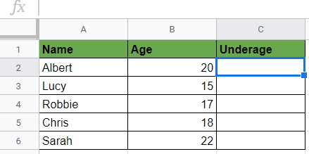
In this example, we want to write a formula to automatically calculate which students are underage in our list.
- Select the first cell where you want your array to start! For this guide, I will be selecting C2.
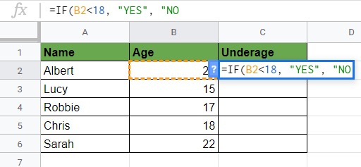
- To count who is underage, we will use an
IFformula that returns “YES” if the age is under 18 and returns “NO” if it is over 18. TheIFformula we would use in a single cell:=IF(B2<18, "YES", "NO").
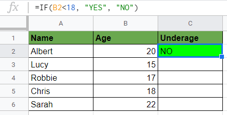
- If we hit Enter to this formula, and it returns the result for the first student. It says “NO” which means that this student is not underage. (To make it more visible, I added conditional formatting to the whole column C to mark the cells red when the result is “YES” and mark them green when the result is “NO”).
- Now we want to change this formula into an
ARRAYFORMULAto apply the calculation to the whole column. We wrap the formula into anARRAYFORMULA. You can write it manually or press Ctrl+Shift+Enter to do it:=ARRAYFORMULA(IF(B2<18, "YES", "NO"))
- Now we must change the single cell reference into a range reference where we want to extend the calculation. So we replace the B2 reference into a column reference B2:B to apply it to the whole column B. We have to change the reference in the following way:
=ARRAYFORMULA(IF(B2:B<18, "YES", "NO"))
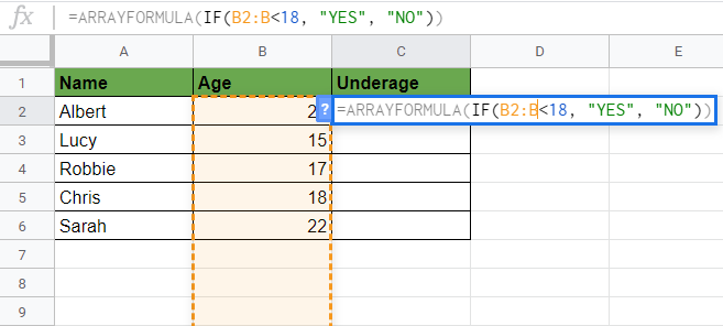
- Hit Enter, and you can see the entire column filled with the result.

- Great! We have filled only one cell and returned the result for the whole column! You can experiment with how automated it works. Add a new student to the table, and the Underage column will be filled automatically!
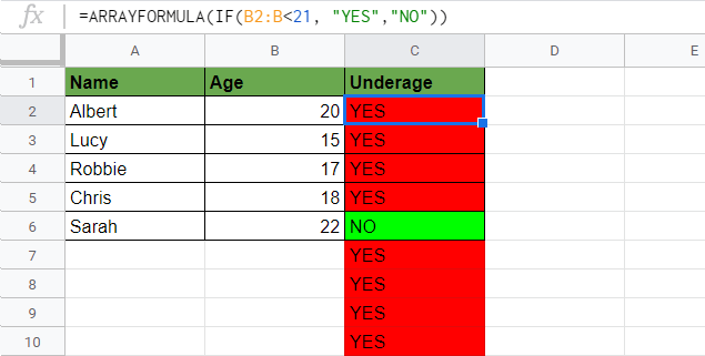
- Now let’s change our condition and consider people under 21 years underage. We only need to change the condition (18 to 21) in the first cell:
=ARRAYFORMULA(IF(B2:B<21, "YES", "NO")). Thus the formula recalculates the whole range. It is very flexible!
That’s it, well done! You can now use the ARRAYFORMULA function together with the other numerous Google Sheets formulas to create even more powerful formulas that can make your life much easier. 🙂