How to Use SORT Function in Google Sheets

The SORT function in Google Sheets is useful to sort and return the rows of a range by the values in one or more columns in ascending or descending order.

Sorting is one of the most important and most frequently used features there is in Google Sheets.

It is possible to access sorting from the menu bar in Google Sheets, but it can also be typed into a cell, like other functions. The difference between the two solutions is that while the menu function sorts the original range itself, the SORT formula sorts the range to a new range of data with the new, sorted output, and the original data remains unchanged.

So using the SORT function instead of the menu bar makes sense in the following situations:

• When you want to keep both the old, unsorted, and the new, sorted ranges.
• When you want to use it inside other functions. For example, the LOOKUP function only works with sorted data.

The SORT function is used to sort the rows of a given range by the values in one or more columns. We can sort either in ascending or descending order. It also allows us to add multiple criteria across columns.

 

 

The Anatomy of the SORT Function

The syntax of the function specifies how we should work with it. The syntax of the SORT function looks like this:

=SORT(range, sort_column, is_ascending, [sort_column2, is_ascending2, ...])

Let’s break this down and understand what the SORT function and its attributes mean:

• = the equal sign is how we start any function in Google Sheets.
• SORT is our function. We will have to add the following arguments into it for it to work.
• range is the data to be sorted.
• sort_column is the index (number) of the column in the range. The sort_column can also be a range outside of range by which to sort the data.
• is_ascending is TRUE or FALSE, indicating whether to sort sort_column in ascending order. TRUE sorts in ascending order and FALSE sorts in descending order.
• sort_column2 , is_ascending2 are optional additional columns and sort order flags beyond the first, in order of precedence.

Without using the optional values, you can sort a data set by one column. Using two or more additional sorting arguments will enable you to sort by multiple columns.

---

⚠️ Notes to Make Your SORT Function Work Perfectly

1. You can sort by text and number values as well.
2. When sorting by text values, the alphabetical order (A-Z) means ascending order. We define the opposite (Z-A) as descending order.
3. The sort_column argument should include one single column that covers all the existing rows within the range.
4. The cell range where we want to put our new sorted data should be totally empty. This means that the same amount of rows and columns as the original data should be available next to and below the cell where we write the formula. If there are non-empty cells in this area, an error message is returned by the SORT function.
5. If you use the SORT function with only giving the range, it will automatically sort the range based on the first column, in ascending order.

 

 

A Real Example of Using SORT Function

Let’s look at some examples of how to use the SORT function in Google Sheets.

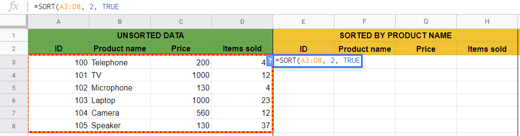
We are going to work with the following example data set containing a list of products with several columns of their details (ID, name, price, number of sold items).

 

---

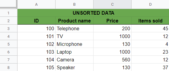
Sort by One Column

Say we want to sort the products by their names alphabetically.

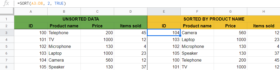
It’s a simple case where we want to sort the products by the values of one column. We have to define the variables in the SORT function:

• range is the whole area where the products are located, which is A3:D8 in the example.
• sort_column is the column of Product name, so it is the second column in the data set.
• is_ascending should be TRUE, because we want to have an A-Z order.

The following formula will do the job:

=SORT(A3:D8, 2, TRUE)

As a result, we get a new table with the same products but sorted alphabetically.

 

 

You can see how to write this function step-by-step below in the last section.

So we have seen how the SORT function works in the simplest version, but there are more options to use it on our data set. Let’s look at some other ways of how to use SORT function in Google Sheets!

You may make a copy of the spreadsheet using the link I have attached below and try it for yourself:

---

Sort by Multiple Columns

So far we only used the mandatory arguments of the SORT function, and we sorted our data set by one column.

We can see from the syntax of the SORT function, that it is possible to sort by multiple (two or more) columns with the additional arguments.

We can write a SORT function with more arguments in the following way:

=SORT(A3:D8, 3, TRUE, 4, FALSE)

Let’s see what happens here!

First, the formula sorts the range by the third column, by the prices in ascending order (because is_ascending is TRUE).

The secondary sorting argument comes in where the first sorting results in a tie. In the example, where the products have the same price, they are then sorted by their columns of “Items sold” in descending order (because is_ascending is FALSE).

 

 

For example, the speaker and the microphone have the same price, so after the first sorting, the formula also sorts them by their number of sold items. The same applies to the laptop and TV.

Now let’s change the order of the arguments, and firstly sort by the fourth column in descending order, then sort by the third column in ascending order:

=SORT(A3:D8, 4, FALSE, 3, TRUE)

In this case, the primary sorting is based on the number of sold items, and if that is the same for two or more products, then they are sorted by their prices in ascending order.

 

 

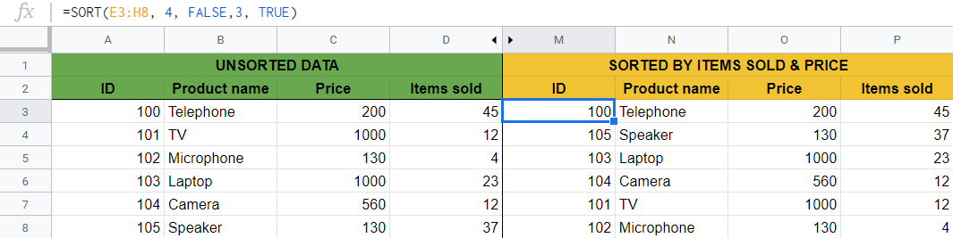
You can see that we get a totally new order with this formula. That’s how the order of the arguments matters.

---

Sort Based on a Range Outside the Sort Range

In the previous examples, we sorted the whole range of our data. It means that the content of one row has never changed. None of the values of the products have been mixed, only their order has been sorted.

Let’s look at an example where we only want to sort a part of the whole data and we want to use a column reference which is not in the range that we want to sort.

Obviously, we don’t want to mix up the product names and their prices, but say we would like to assign new IDs to the products. We would like to assign the smallest ID to the first product when sorted alphabetically and so on.

In formula words, we would like to sort the ID column by the name column in ascending order starting from the cell B2.

 

 

The range is not the whole data of the products now, but only the column with the IDs since we only want to sort these values.

In this case, we can’t write the sort_column as the number of the column, because it is not part of the range to be sorted. We have to define a column reference on which we want to base our sorting. Here we want to use the values of the name column, which are in the cells C2:C7.

Taking this into consideration, the formula we should write in the cell B2 is:

=SORT(A2:A7, C2:C7, TRUE)

After hitting the ‘Enter’, we have the newly sorted column of IDs. Meanwhile, the rest of the data set did not change, so we have successfully assigned new IDs to our existing products.

 

 

Be aware that it is not possible to delete the column of the old IDs here. It is because the new IDs depend on their column, and there will be an error if you try to remove the old column.

As we mentioned above, using the SORT function for such a case is only useful if you want to keep both the old and new columns. If you only need the new, sorted column, it is better to use the sorting options of the menu bar.

 

 

How to Use SORT Function in Google Sheets

Let’s get back to the example of sorting the products by their names alphabetically and see how to write the SORT function step-by-step.

1. Before starting it, we have to decide where we would like to put our sorted data. There should be an available empty area with the same number of rows and columns as the original data. For the purposes of this guide, we will make sure that the area E3:H8 is empty before starting to work with the SORT function:

 

2. We will write our SORT formula in the cell E3 (as this is the cell where we want to start our new sorted data). So click into the cell and start typing =SORT(.

 

3. After the opening bracket, we have to add the first argument. The range will be the whole unsorted data set, so the range of A3:D8.

 

4. We separate the values inside the function with commas ‘,‘.

 

5. The sort_column is the second column with the product names, so we have to write 2 as the second argument.

 

6. We want to sort them alphabetically which means ascending order, so is_ascending  should be TRUE.

 

7. We are not going to use the optional sort_column2, is_ascending2  values because we only sort by one column.

 

8. After we have written all the necessary variables, we have to close the brackets ‘)‘. Therefore we have to write the following formula in the cell E3 and then hit Enter:

=SORT(A3:D8, 2, TRUE)

 

The result is a new range with the products sorted in ascending order by the second column. We have all the products with their details on a new sorted list.

 

That’s it, well done! You can now use the SORT function together with the other numerous Google Sheets formulas to create even more powerful formulas that can make your life much easier. 🙂