Query Function with Multiple Criteria in Google Sheets

This guide will explain how to use the QUERY function with multiple criteria in Google Sheets.

Using multiple criteria in the QUERY function allows users to perform more advanced filtering.

Google Sheets has several ways to filter and select data in a range. The most powerful function for this task is the QUERY function. The function allows you to use logical operations and other built-in Google functions together using a specialized query language.

Let’s begin with a simple use case where we can filter data from a table using the QUERY function.

Suppose you have a list of products that are in your inventory. You want to create a set of these items to promote on social media. You have several criteria that will help determine which items you should prioritize when promoting. How can we filter our dataset in Google Sheets?

With the QUERY function, we can add multiple criteria using the keywords ‘AND’ and ‘OR’.

This use case is just one way to use the QUERY function in Google Sheets. Since the function is so powerful, you can use the QUERY function to filter various data types. The function supports all types of values, including text, Boolean, and numeric data.

Now that we know when to use multiple criteria with the QUERY function, let’s dive into how we can use it on an actual sample spreadsheet.

A Real Example of Using Query Function with Multiple Criteria in Google Sheets

Let’s take a look at a real example of a spreadsheet that uses the QUERY function with multiple criteria in Google Sheets.

In the example below, we have a table with product information. Each product has a unique product ID, a brand, price, and discounted price. 

From this list of products, we want to create several collections based on several criteria. In this example, we’ll consider a ‘cheap’ product any product worth less than $100.

In the spreadsheet below, we’ve created two additional tables that use certain criteria to filter products from our original table.

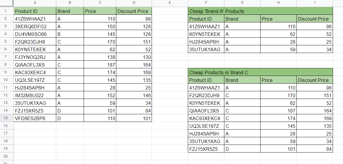
To get the results for Cheap ‘Brand A’ Products, we’ll use the following formula:

=QUERY(A2:D15, "SELECT A, B, C, D WHERE B CONTAINS 'A' AND D < 100")

Our query above uses two criteria: B CONTAINS A and D < 100. These two criteria are placed after the ‘WHERE’ keyword. Since we only want entries where both conditions are met, we use the keyword ‘AND’.

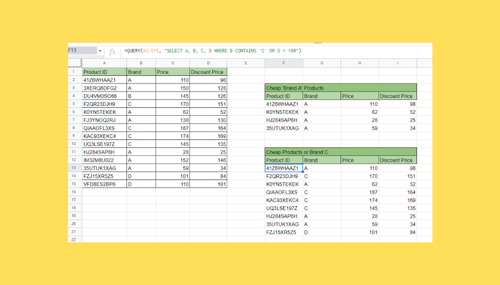
To get the results for ‘Cheap Products or Brand C’, we just need to use the following formula:

=QUERY(A2:D15, "SELECT A, B, C, D WHERE B CONTAINS 'C' OR D < 100")

Since we want entries that are either ‘cheap’ or are part of Brand C, we use the ‘OR’ keyword instead.

You can make your own copy of the spreadsheet above using the link attached below. 

If you want to try using the QUERY function with multiple criteria in Google Sheets, let’s start writing it ourselves!

How to Use Query Function with Multiple Criteria in Google Sheets

This section will guide you through each step needed to start using the QUERY function with multiple criteria in Google Sheets. You’ll learn how we can use the ‘AND’ and ‘OR’ keywords to control how the QUERY function uses our criteria.

Follow these steps to start using the QUERY function:

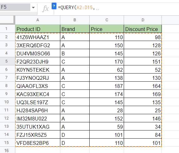
1. First, select the cell that will hold our QUERY function. In this example, we’ve added new headers for our ‘Cheap Brand A Products’ collection. We’ve chosen cell F5 as the starting cell for our query result.
   
2. Next, we just need to type the equal sign ‘=‘ to begin the function, followed by ‘QUERY(‘. For our first argument, we’ll select the range A2:D15.
   
3. Next, we’ll need to construct the actual query we’ll use. Every query starts with the ‘SELECT’ keyword, followed by the columns you want to include in the final result. In this example, we will select columns A through D.
   
4. Next, we’ll add the ‘WHERE’ keyword to our query. In our WHERE clause, we’ll add the necessary criteria. In this example, we’ll add criteria that checks if the brand of the product contains the string ‘A’ and checks if the discounted price is less than $100.
   
5. Hit the Enter key to evaluate the QUERY formula. You should now see the entries that fit your query’s criteria.
   
6. Instead of using the ‘AND’ keyword, you can use the ‘OR’ keyword to return entries that fit either of the listed criteria.
   
   

This step-by-step guide should be all you need to start using multiple criteria in your query function in Google Sheets. In conclusion, our guide shows how to use the ‘OR’ and ‘AND’ keywords in the WHERE clause of your query.

The QUERY function is just one way you can filter and transform data in Google Sheets. With so many other Google Sheets functions available, you can surely find one that works best for your data.

Are you interested in learning more about what Google Sheets can do? Subscribe to our newsletter to find out about the latest Google Sheets guides and tutorials from us. 

Get emails from us about Google Sheets.

Our goal this year is to create lots of rich, bite-sized tutorials for Google Sheets users like you. If you liked this one, you'd love what we are working on! Readers receive ✨ early access ✨ to new content.

Subscribe