How to Use ADDRESS Function in Google Sheets

The ADDRESS function in Google Sheets is useful if you want to return a cell’s address in the form of a text.

In other words, the function returns a cell reference or address as a text or string as per the specified row and column numbers. 

The Anatomy of the ADDRESS Function

The way we write the ADDRESS function is: 

=ADDRESS(row, column, [absolute_relative_mode], [use_a1_notation], [sheet]) 

Let us help you understand the context of the function:

• The equal sign =  is how we start any function in Google Sheets.
• ADDRESS() is our function. We need to add two attributes, namely the row and column, to make it work correctly. The other three attributes are optional, namely the [absolute_relative_mode], [use_a1-notation], and [sheets].
• The row is the row number of the cell reference.
• The column is the column number of the cell reference. For example, “A” is column number “1”.
• The [absolute_relative_mode] is the indicator of whether the cell reference is row or column absolute. This attribute is optional. 
• The  [use_a1-notation] is an expression used to indicate what style notation to display the cell reference in. This attribute is optional. 
• The [sheets] is to indicate the name of the sheet of the cell reference. This attribute is optional. 

Let’s have a more detailed understanding of what [absolute_relative_mode] and [use_a1-notation] mean.

Absolute Relative Mode:

This attribute is to determine whether the cell reference’s address would be relative or absolute.

Relative and absolute references behave differently when copied and filled to other cells.

Relative: changes when a formula is copied to another cell. 

Absolute: remain constant, no matter where they are copied to.

Here are the references:

This attribute is optional; hence it would be “1” by default.

Use A1 Notation:

This attribute is to determine how the cell reference’s address would be displayed.

Here are the references:

Let’s take an example

Example 1:

By using the ADDRESS function, the formula returns the cell address of “lemon” in the form of text.  

As mentioned, without inputting the [absolute_relative_mode] attribute, it would be 1 by default, showing row and column absolute. 

Example 2:

By adding false as the [use_a1_notation] attribute, the cell reference address is displayed in the form of “R2C[1]” instead of “A$2”.

Besides, inputting 2 as the [absolute_relative_mode] attribute displays the row as absolute. 

Do note that the value within the [] square bracket indicates that it is relative.

Example 3:

By adding “Sheet1” into the formula, it will display which sheet the cell reference address is at.

A Real Life Example of Using ADDRESS Function

Let’s use a real-life situation to utilize the ADDRESS function and combine all the components mentioned so far in practical use and show you how powerful this function can be!

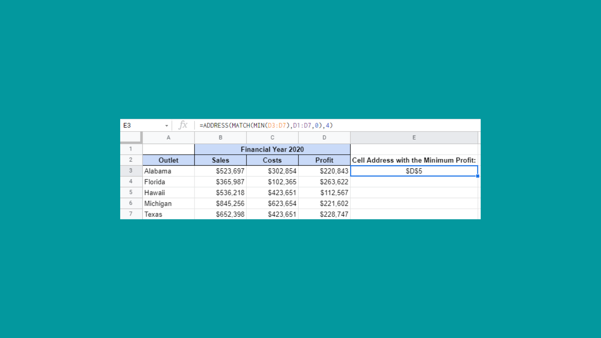
In this example, we use the ADDRESS function to determine which outlet has the minimum profit. 

As shown, we incorporated MATCH and MIN  functions to evaluate which outlet needs further inspection or is no longer generating a profit. 

How to Use ADDRESS Function in Google Sheets

1. Simply click on the cell that you want to write down your function at. In this example, it will be E3.

2. Begin your function with an equal sign =, then followed by the name of the function, ADDRESS, then an open parenthesis (.

3. We will then add the MATCH and MIN functions. The MIN function is to find the smallest numeric value in the range of profits from all outlets. The MATCH function would help match the smallest numeric value returned to the range of profits.

4. We will then select D3 to D7, as this is the range of profits we will want to search the smallest numeric value from. The colon : is added to include all cells between the two endpoint cell references.

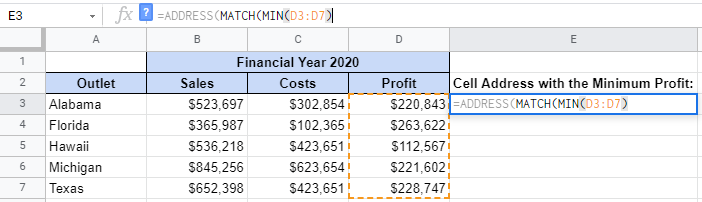
5. Furthermore, we need to add a comma , to separate the lookup_value from our next attribute, lookup_array. We will then select D1 to D7, as this is the range of cells being searched to match the lookup_value.

6. Next, add another comma , to separate the lookup_value from our next attribute, match_type.  In our case, we would like to find the first value that is exactly equal to the lookup_value. So we will add 0 for this expression.

7. We then add a closing bracket ) to close the MATCH function. Don’t forget to add a comma , to separate the row from column. To finish off the formula, we will add 4 as the column of cell reference is in Column D.

Our final formula would look like this:

=ADDRESS(MATCH(MIN(D3:D7),D1:D7,0),4)

8. After the following steps, your input should look like this:

9. To give you a summary of how the formula was formed, here is a visual guide:

You may make a copy of the spreadsheet using the link attached below and try it for yourself:

That’s about it! You can now use the ADDRESS function in Google Sheets together with the other numerous Google Sheets formulas to create even more powerful formulas that can make your life much easier.

Get emails from us about Google Sheets.

Our goal this year is to create lots of rich, bite-sized tutorials for Google Sheets users like you. If you liked this one, you'll love what we are working on! Readers receive ✨ early access ✨ to new content.

Subscribe