Getting dynamic sheet names in Importrange is useful, especially when we are working on a large database, and we want to choose specific data from a tab in Google Sheets.
There are other Google Sheet guides out there that say, using an INDIRECT function as a range_string in IMPORTRANGE is effective. Many users have tried this method, but they were unsuccessful. Why? It is because of the wrong usage.
At this point, you may be confused about why we are talking about Importrange in Google Sheets. When do we use that? Or, is it helpful?
Well, let’s say you are working on two sheets in one Google Sheets file. We name it, spreadsheet A and B, respectively. In spreadsheet A, you’ve inserted a lot of spreadsheets. While working on spreadsheet B, you remembered that the information you need is in cell D1 of spreadsheet A. This is where you will need to get dynamic sheet names in Importrange to get the data that you need.
In this guide, I’ll show you how you can get started and help you create your dynamic sheet names in Importrange with Google Sheets.
⚠️ Note
Using IMPORTRANGE function can be a slow formula because we’re using it to connect to another sheet to retrieve data. It’s best practice to minimize the number of these external calls wherever possible.
Additionally, when your data starts to get big (say around 10,000-20,000 rows), the IMPORTRANGE formula will just get stuck at the Error Loading data... message. We will address how to fix this with another post in the coming weeks. Subscribe to our newsletter to be notified when it is published.
Let’s dive right in. 🤜
How to Get Dynamic Sheet Names in Importrange in Google Sheets: 10 Steps
- Jump into your Google Sheets and prepare your data. It’s best to have more than one sheet so you could see how the
IMPORTRANGEreally works. For this guide, I went ahead and listed the sales for January and February. That would be one sheet per month.

- Great! Now that you’ve prepared your data, you have to add another sheet that will serve as our ‘master sheet’. This is where we will place our formula and perform data validation. This is what your spreadsheet should look like:

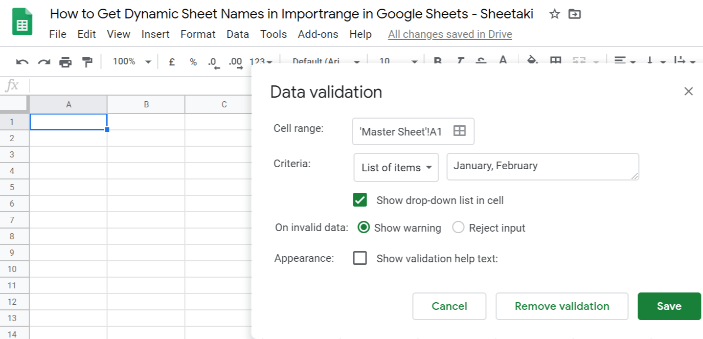
- Now that you have three sheets in total let’s get into action! So for the next step, we will make a drop-down menu so that we don’t have to type down the name of each month whenever we search for data. To do this, we have to click on an empty cell to make it active. For this guide, I’ll be selecting cell A1 on the Master Sheet tab.
- Next, press the right-click on your mouse, then scroll down to Data validation that is found on the last of the options, then click it.

- Then, on the criteria drop-down menu, choose ‘List of items‘. List down the names of your tabs. In my case, I’ll list down January and February. Separate those with a comma. Then save. It should show up something like this:
- Wow! You’re getting it! Good job! Now, we have to name our range. To name it, we will go to the sheet where our database is. Then, we select the range that we want to include in the search. After that, we click on Data, found in between Format and Tools option tabs. Then, look for Named ranges and click that. By default, you will see ‘NamedRange1‘. Change it to your desired name range, then click Done. In my case, I went to my January tab, selected the range A1:B6, then named my range with the name of the month itself, January. Simply do these steps until you reach your last sheet tab. It should look somewhat like this:

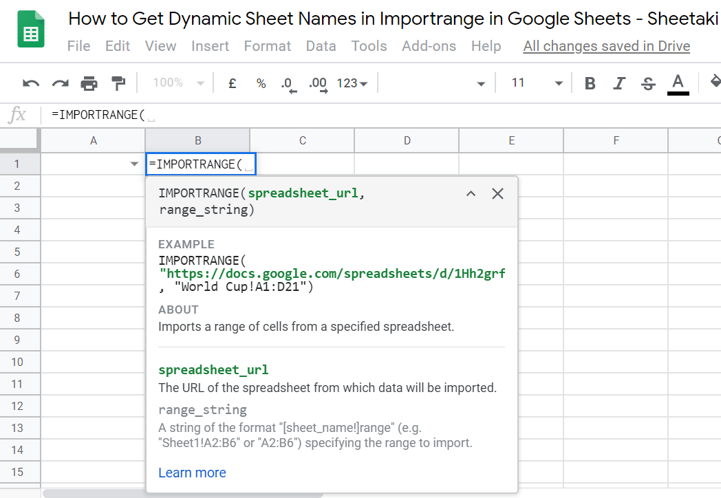
- Now that we’re done naming our range, we’re now more than ready to write our formula. Select an empty cell to activate it. For this guide, I selected B1. Then, we write our function, which is the
IMPORTRANGE, followed by an open parenthesis ‘(‘. Wait for the auto pop-up message because that will serve as our extra guide.
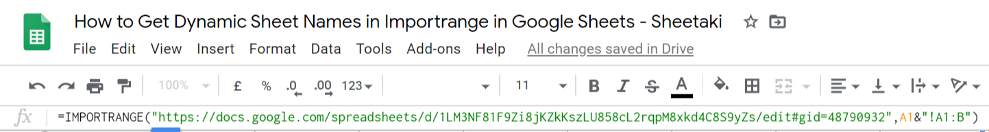
- Great! Next, we have to copy+paste the spreadsheet URL. Then select the drop-down menu that we made earlier. For this guide, I will select A1, then follow it up with an ampersand (&) symbol.
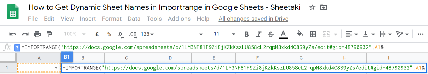
- Add an exclamation point (!). This would tell that we are referencing another tab/sheet. Then, we select the range that we are trying to reference. We selected the range A1:B. Enclose all these in a quote-unquote symbol (” “).

- Lastly, close your formula with a close parenthesis “)“. Then hit on the ‘Enter’ key. Whenever you select a specific item from your drop-down menu, you should see the necessary data being loaded. Take note that it may take a few seconds. This is because, as mentioned above, the
IMPORTRANGEis generally a slow function primarily when we use it to connect with another sheet and intend to load the data from it. We will discuss quicker ways on how to go about this in a future post.
Voila! ✨

That’s pretty much it. Feel free to make a copy of the example spreadsheet above to try and see how it is done. The most important lesson is you should have fun doing it.
Let me know how it goes down below, and I’ll try my best to reply to you and help you or even have a look at some of your finished dynamic sheets.