How to Use IF Functions in Google Sheets

The IF function is useful if you want to test whether a certain condition is true or false.

Let’s take an example.

Say we have a dog and let’s call it Spencer. 🐶

Our first condition is whether Spencer is an animal. Since Spencer is really a dog which is some kind of an animal, we can apply the IF function on our condition then it would return the value of True since Spencer is an animal.

What if our condition is whether Spencer really is a duck? Again if we apply the IF function, the function would return a value of False because Spencer is not a duck.

That’s all really how the IF function works. It’s simple and models perfectly our simple decision-making process.

You know what else it can do?  You can even create an IF-ception (a play on words with the movie Inception). I’m kidding. Basically, you can create an IF function in an IF function. It’s called a nested IF where one IF functions nests under the other.

Let’s call Spencer again! 🐶

Say we have our first condition that Spencer is an animal, our first IF function will return a value of true. Now right away we can have another condition which asks IF Spencer is really an animal, then is Spencer a dog or is Spencer a cat?

If Spencer is a dog then it would return a final value of true ignoring the condition that we make Spencer out to be a cat even though he is an animal.

You see what I just did?

I just added another IF function right under our original IF function. This is called branching and you can do it as many times as you like and go as deep as you like with the branches.

It is one of the many powerful tools to have in your Sheetaki arsenal to solve a lot of our business data entry problems and shave half of your data entry time.

Let’s dive right into real-business examples where we will deal with actual values and how we can write our own IF function in Google Sheets to compute those data.

The Anatomy of the IF Function.

There is a term to how we call writing a function and that term is called syntax. It’s pretty commonly used everywhere.

So the syntax (the way we write) the IF function is as follows:

=IF(logical_expression, value_if_true, value_if_false)

Let’s dissect this thing and understand what each of these terms means:

• = the equal sign is just how we start off any function in Google Sheets.
• IF() this is our IF function. We will have to add our logical_expression, value_if_true, value_if_false inside the brackets for the function to work.
• logical_expression is the condition that we want to test to see if it is true or false.
• value_if_true is the operation (the work to be done) that we want to carry out if the said argument is tested to be true
• value_if_false is the operation ( the work to be done) that we want to carry out if the said argument is tested to be false.

Note: The value_if_false part is optional and you do not have to write for it. However, you must specify the first two components (logical_expression and value_if_true) for the function to process correctly.

Now it may look a little complicated for some but don’t worry. We will go through it and subsequently practice applying it.

A Real Example of Using IF Function.

Take a look at the example below to see how IF functions are used in Google Sheets.

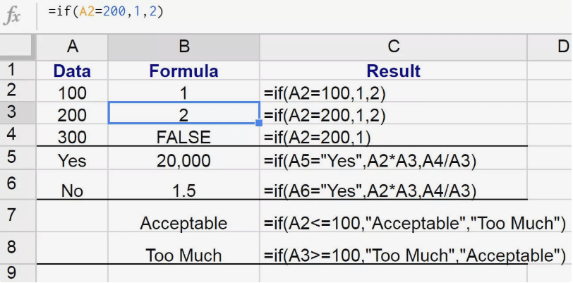
As you can see in the image above, the IF function is:

=if(A2=200,1,2)

Here’s what this example does:

• We have actively selected the cell (or box) under B3 (B column, 3rd row) and we want to use the IF function to find out the value needed to be inserted into B3.
• Our condition is that if in cell A2 the value is and equals to 200 (A2=200), then output the value of 1 if the condition is found to be true or output the value of 2 if the condition is otherwise found to be false.
• As you can see above the value ‘2’ was inserted into our selected B3 because A2 did not equal to 200.

Simple right?

How to Use IF Function in Google Sheets.

Unlike Excel sheets where you have like a “dialog box” to enter a function, Google Sheets has an auto-suggest box which pops-up with the name of the function that you’re trying for. This is pretty handy.

Here’s how you start using IF Function in your own Google Sheets:

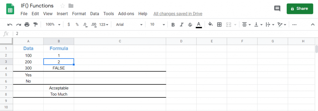
1. Simply click on any cell to make it the active cell. For the purposes of this guide, I’m going to choose B3 as my active cell.

2. Next, simply type the equal sign ‘=‘ to begin the function and then followed by typing the name of the function which is our ‘if‘ (or ‘IF‘, whichever works).

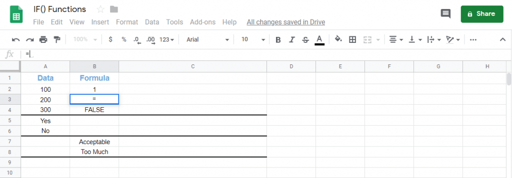
3. Great! Now you should find that the auto-suggest box appears with the names of the functions that all start with IF.

4. The one we want is our IF function. So make sure to click on the IF function name. If you get a huge box with text in it, simply hit the arrow on the top right-hand corner of the box to minimize it. You should now see as follows.

5. Now what you need to do is click the cell that you want to want to use the IF Function on as the condition. I will be using A2 to find out if the value in A2 is 200 then I want the function to output 2 into B3 otherwise output 1 into B3.

Tip: The cell (or box) you select has a fancy name called the cell reference which means that the cell is used as a reference for the function.

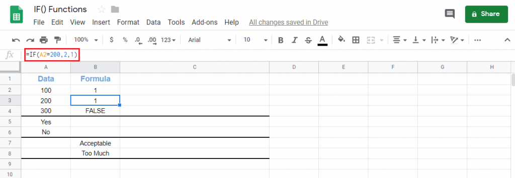
6. Next, we need to complete our function so that it can properly work. So type the equal symbol ‘=‘ after the ‘A2‘ in the IF function and then followed by the number, which in this case, will be ‘200‘ because I want to test whether A2 is 200.

7. Following the ‘200‘, enter a comma ‘,‘ to complete the condition. Then type the true value, which will for me be ‘2‘. Follow up with a comma again.

8. Following the ‘2‘ we had entered for as true value, type the false value, which will (for me) be ‘1‘. Do not follow up with a comma here. Your function should now look similar to mine:

9. Finally, just hit your Enter key. You’ll find that, if you followed my steps, that the value 1 should appear in cell B3. This is because the value in cell A2 does not equal to 2, hence it takes the false value in our function and inserts it into our B3 cell. That’s it.

That’s it. Well done! 👏🏆

You can now use IF functions in Google Sheets together with the other numerous Google Sheets formulas to create even more powerful scripts. 🙂

Get emails from us about Google Sheets.

Our goal this year is to create lots of rich, bite-sized tutorials for Google Sheets users like you. If you liked this one, you'll love what we are working on! Readers receive ✨ early access ✨ to new content.

Subscribe