


The XIRR function in Google Sheets is used to calculate the internal rate of return on investment based on a specified series of potentially irregularly spaced cash flows.
Table of Contents
This function is used to find the internal rate of return. The internal rate of return is a metric in financial analysis that refers to the expected annual rate of growth or an investment, based on certain factors. This special form is used when the cash flows come in at different times, affecting the profitability of the project,
The IRR is useful because it helps you estimate the profitability of certain projects and investments. It is an ideal tool to use to study and compare different rates of annual return in a period of time. The XIRR function, keeping in mind different cash flow dates, make this calculation a bit more accurate rather than the IRR.
Let’s look at an example.
You want to choose what investment to pursue for your company. You have the information about the cost of the investment, the cash flows it will generate, and any growth in the next years.
How should we go about this problem?
The XIRR function needs you to set up a table of cash flows and the dates when they come in. This calculation can help you determine if your project will be profitable or not. This is usually compared to the company’s cost of capital. If the IRR is greater than the cost of capital, the project will make a profit for the company.
The Anatomy of the IRR Function in Google Sheets
The syntax of the XIRR function is as follows::
=XIRR(cashflow_amounts, cashflow_dates, [rate_guess])
Let’s have a look at each part of the function to understand what is going on here:
=is the equals sign that starts off any function in Google Sheets.IRRis the name of our function.cashflow_amountsis the input of the function. Choose an array or range containing the income or payments associated with the investment.cashflow_datesis the range of cells containing the dates according to the detailed payments incashflow_amounts.rate_guessis an optional input. It is an estimate for what the internal rate of return will be.
You should also note that the perspective you are solving the problem from also matters.
If you are the owner of the investment, the cashflow_amounts will represent income, so they should be positive.
If you are the perspective of someone making a loan repayment, the cashflow_amounts will represent payments, so they should be negative.
If your project returns cash flows at a regular interval, then use the IRR function instead.
A Real Example of Using the XIRR Function
Let’s look at the example below to see how to use XIRR function in Google Sheets.
Calculating the Internal Rate of Return in Google Sheets
This is a simple problem. We want to find the internal rate of return for a certain project. Here in the example, the cash flow is laid out.
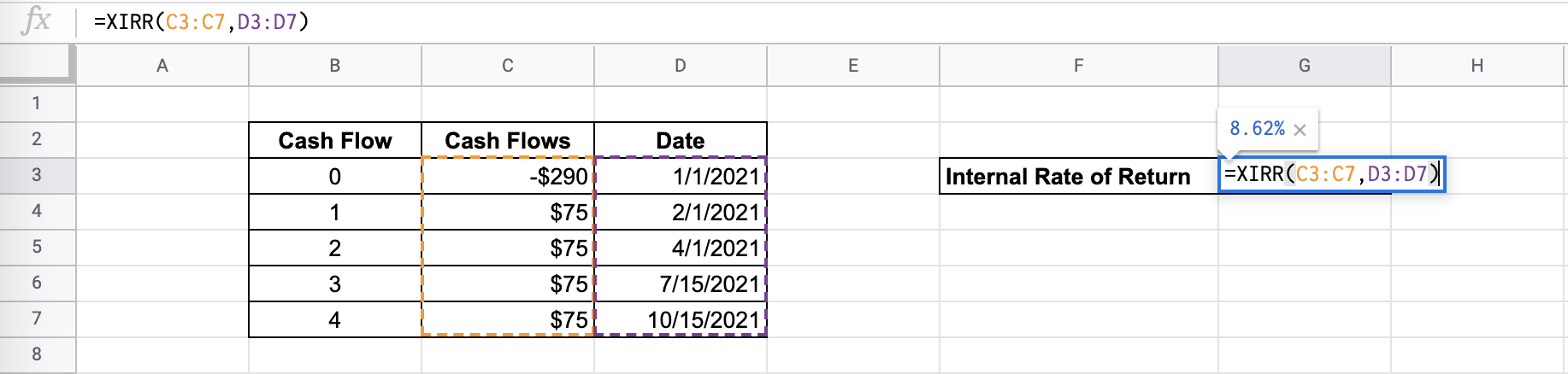
The function takes three arguments. So in the equation, it will look like:
=XIRR(C3:C7,D3:D7)
As a result, we get 8.62%.
This simple problem can be practiced to perfection. Use the link below to get a copy of this problem set:
How to Use the XIRR Function in Google Sheets
In this section, we will show you a step-by-step process on how to use the XIRR function in Google Sheets.
In this problem, we will be comparing three different projects. The information that you have is laid out over three different cases. They are all projects that are not easy to compare at first glance, because they have different costs and different cash flows to offer the company.
You know that IRR is usually used to compare projects that run in the same period of time. Given that IRR does not consider the cost of capital in the calculation, this is a quicker and simpler but less accurate way to compare projects.
It’s up to you, as the project manager, to decide which project will benefit the company the most. You have decided to use the IRR to compare these projects.
Calculating and Comparing IRR in Google Sheets
- To begin, click on a cell to make active, which you would like to display the XIRR. For the guide. The XIRR will be in Cell G3.

- Next, type the equal sign ‘=’ to start writing the function. Follow this with “XIRR” or “xirr” – Google Sheets functions are not case sensitive, so either is fine.

- The auto-suggest box will create a drop-down menu. Select the
XIRRfunction by clicking it. It is the first to pop up on the list, but take care to choose the correct function.
- After the opening bracket ‘(‘, you will add the range attribute. Drag your cursor over the entire cash flow column.

- Next, drag your cursor over the entire cash flow column.
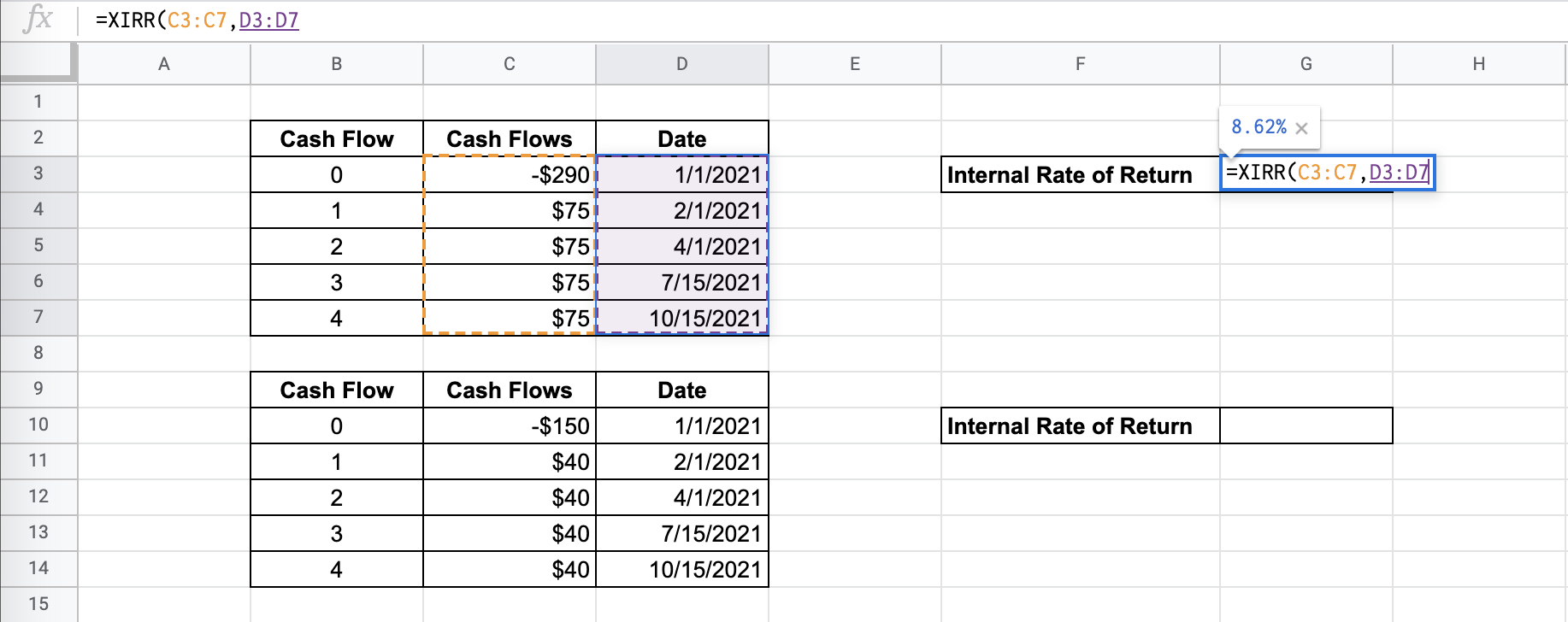
- You will notice that there will be a preview of the result when you complete the inputs. Hit enter! You can now see the IRR of the project you are working on.

- Do the rest of the set – and make your decision as a project manager!
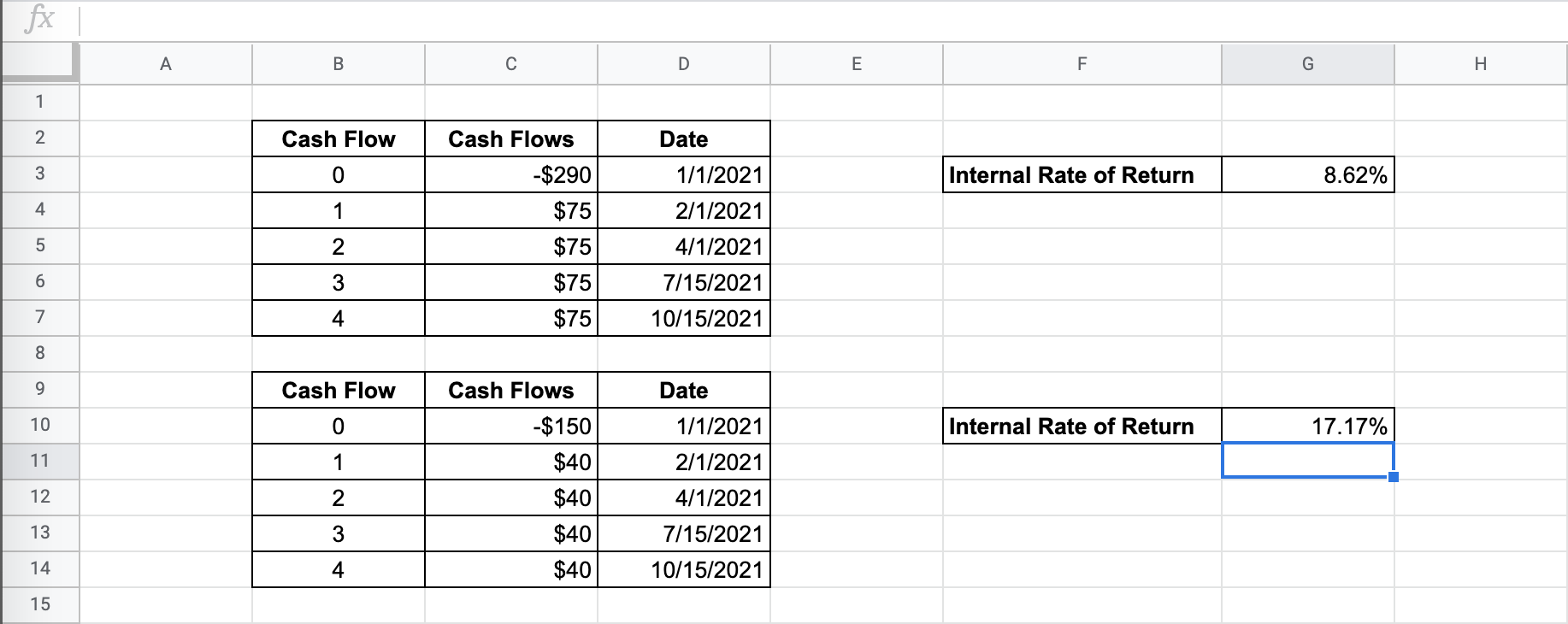
Given a practical problem where you should completely solve for the return on investment, use XIRR to find and compare the rates of return of the other projects.
And there you have it – you can now use the XIRR function in Google Sheets together with the other numerous Google Sheets formulas to create even more effective formulas.


