How to Hide Columns or Rows From Certain Users in Google Sheets

There is no one-stop solution in Google Sheets to hide columns or rows from certain users alone. It is either hidden or visible, and will be the same way for all users having access to the spreadsheet. Is there a workaround, then? The short answer is yes.

We can leverage the IMPORTRANGE() function to achieve the desired result. The IMPORTRANGE() function in Google Sheets is useful to import a range of cells from a specified spreadsheet.

IMPORTRANGE() function helps you bring data from one sheet to another. So, if you want to hide columns or rows from some users, just import only the relevant ones to a new spreadsheet and share them with the concerned users. In this guide, we will look at how to use the function to hide or show select columns or rows from certain users.

Let’s take an example.

A Real Example of Hiding Columns or Rows From Certain Users

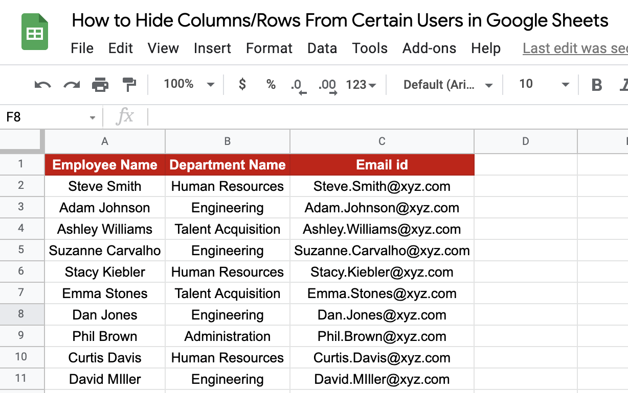
Take a look at the below data where the payroll department of a company has captured employee details:

The above data is sensitive in nature since it includes salary information. While the Human Resources team will have the entire information, the company would like the administration department to have access to this data but for the salary. Hiding the column will not work since it will stay hidden for all users accessing the sheet.

This is where they can use the QUERY() with IMPORTRANGE() function to their benefit. The function enables them to pull only the required columns into a new sheet, and they can provide the administration department access to this new sheet.

And once you are done with populating the required columns in the new sheet, go ahead and share this sheet with the users you want to limit from seeing the full data. Check out how the results change when you use a different query. You may copy the spreadsheet using the link below:

Amazing! Let’s take a closer look at the components of the function and then proceed to a detailed walkthrough of using QUERY() with IMPORTRANGE() function to hide columns or rows from certain users only.

The Anatomy of the Importrange Function

So the syntax (the way we write) of the QUERY() with IMPORTRANGE() function is as follow:

=QUERY(IMPORTRANGE(spreadsheet_url, range_string), query, [headers])

Let us look at what each term means:

• = to start with a function, we must add this sign.
• QUERY() selects the cell ranges you want to display based on your criteria.
• IMPORTRANGE() imports values from cells (or cell ranges) in a given spreadsheet into your active spreadsheet.
• spreadsheet_url is the link to the spreadsheet where the cells that you want to import currently reside.
• range_string denotes the cells (or cell ranges) that will be imported. This has two parts: the sheet name and the cell ranges separated by ‘!’ and in double quotes ”“. For example, “”Example – Input!A2:D11″”.
• query gives the criteria based on which the data is imported.
• [headers] – optional. The default value “1” is given if your data has headers.

Let us go through in detail on how to hide columns or rows from certain users using the QUERY() with IMPORTRANGE() functions together in Google Sheets.

How to Hide Columns or Rows From Certain Users in Google Sheets

1. Below is the annual salary hike summary for ten employees for a certain department within a company. The director would like to share the information with two sets of audiences. One, the employees themselves, without divulging the final salary hike information. And two, the senior leadership, where the hike will be shown to account for the budget allotted.

2. Now, create a new sheet that you will be sharing with the users who will have restricted visibility to the data.
3. Add only the column headers you want to display to all employees.
4. In the new sheet, click on cell A2. This is where you will enter the formula to bring the required data from the original sheet.
5. Type the equal sign ‘=‘ to begin the function and then follow the function’s name, which is our QUERY() followed by IMPORTRANGE(). Note that you are using the IMPORTRANGE() function to get the data parameter for the query function.
6. The auto-suggest box will appear for each function. Continue by entering the first opening bracket ‘(‘. You should now see it as follows:

5. Copy the original sheet URL and paste it within quotes. And select the entire cell range as the second input. Make sure that the range_string is enclosed within quotes. Once you’ve entered the necessary values, or you’ve done what I did, make sure to close the brackets for both functions, as shown below:

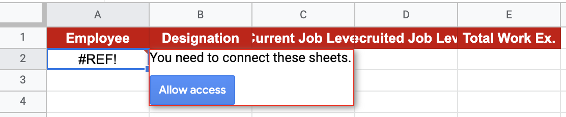
6. If you are prompted to allow access for the import connection, go ahead and click on Allow access.
7. If you’ve done everything correctly, you should have the following output in your new sheet.

How to Absolutely Ensure Restricted Access For Certain Users

Now, a smart user can alter the query parameter to access data that you may not intend to share with them. Just to ensure that your process is fool-proof, you may create an additional sheet that pulls the data from the new sheet you have just created and share that instead. That way, there is no scope for a user to pull any data that is not present in this now “intermediate” sheet.

Of course, if you wish to have a restricted view of multiple groups of users, you may have to manage a larger number of sheets at your end, making it a tad bit cumbersome.

You now have the desired result. Go ahead and share this sheet with all employees. Voila! You are fully equipped to start hiding columns or rows from certain users. 🙂 I recommend experimenting with the QUERY() with IMPORTRANGE() function, combining it with the numerous Google Sheets formulas available, and seeing what you can come up with.

Get emails from us about Google Sheets.

Our goal this year is to create lots of rich, bite-sized tutorials for Google Sheets users like you. If you liked this one, you'll love what we are working on! Readers receive ✨ early access ✨ to new content.

Subscribe