How to Highlight the Smallest N Values in Each Row in Google Sheets

To highlight the smallest n values in each row in Google Sheets is useful to make the cells with the smallest n values in each row easier to identify.

Google Sheets has a built-in feature for formatting cells in your sheets based on whether they meet certain criteria.

This feature is called conditional formatting and is useful not only for formatting cells based on whether they meet certain conditions but for making your sheet visually more appealing, as well. Once you apply conditional formatting across your sheet, you will be able to gain some insight into the data just by looking at it briefly.

Let’s say you sell books and have a sheet that contains information about the number of books sold each day for several weeks 📚📙

And now we want to know which are the days when you had the least sold books each week. We want to highlight these cells by giving them a special background colour so we can easily see these days just by glancing at the sheet.

So how do we do that?

Simple. We should apply some simple dynamic conditional formatting rules and set a style of our choosing.

Let’s first learn how to use conditional formatting in Google Sheets if you don’t know how to do it already.

How to Use Conditional Formatting in Google Sheets

Conditional formatting in Google Sheets is a useful visual tool you can use to change the aspect of cells, rows, or columns (their background colour or the style of the text), based on the values in them and rules you set.

To access conditional formatting, go to the menu and select Format > Conditional Formatting. The ‘Conditional format rules’ toolbar will open on the right.

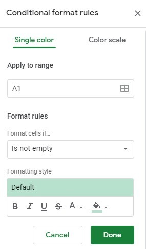
Use this toolbar to set the rules according to which you would want to format your sheet. Every rule you set is an if-then statement, meaning it consists of a condition that needs to be evaluated and a corresponding action if the condition is met.

For example, let’s say that you would want all empty cells to have a red background. The condition would be ‘if the cell is empty’ and the corresponding action would be ‘then the background colour should change to red’. If the rule you set is evaluated as TRUE, the corresponding action will be met and the cell will change its aspect (background colour or text style) according to the style of your choosing.

To apply conditional formatting, you should first set three basic things:

• Range: where would you want to apply conditional formatting
• Condition: what is the criteria that the range should meet in order to be formatted
• Style: how will the cells that meet the condition look once they are formatted

You can choose from default conditions or you can write your own condition. To write your own condition, you should select the ‘Custom formula is’ in the drop-down list of ‘Format cells if’.

In this guide, you will learn how to write a custom formula to highlight the smallest n values in each row in Google Sheets.

Now, let’s go straight into real examples where we will deal with actual values so you can better understand how to highlight the smallest value in each row in Google Sheets and learn how to apply conditional formatting across your sheets.

A Real Example of Using Conditional Formatting to Highlight the Smallest N Values in Each Row in Google Sheets

Now, let’s see how conditional formatting works with real examples and how we can use it to highlight cells in Google Sheets based on our criteria.

So let’s get back to our books! 📚📙

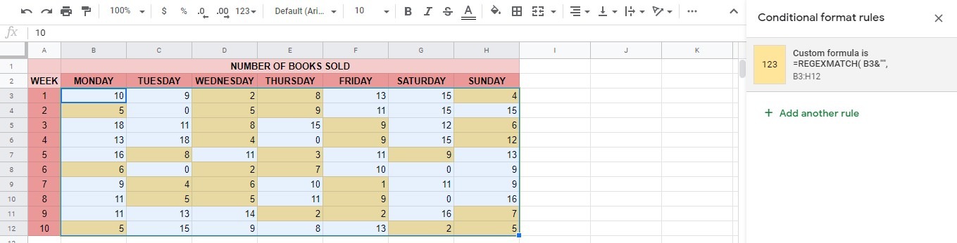
The picture below shows the number of books sold each day for several weeks.

We will use conditional formatting to highlight the smallest n values in each row with a light yellow background. This way we will be able to easily identify days with the lowest numbers of sold books each week.

If you take a look at the list of basic conditions, you will notice that it does not include a condition that could help us, so we should write a custom formula that will highlight the smallest n values in each row.

You might have thought that using the SMALL formula would be practical. However, this is not always an ideal solution. Do you know why? The SMALL formula will return the nth smallest element from a data set. And this is OK if you are looking only for the smallest one number (or two). But what if you would want to highlight the smallest ten numbers in each row in your sheet? You will have to use ten conditional formatting rules using ten SMALL function based formulas.

Since this is not the most practical solution, you will get a formula that will highlight the smallest n values in each row in Google Sheets (including 0 and excluding 0 in the calculation).

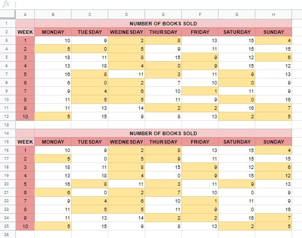
Data is the same in both tables, the only difference being that to the first one we applied the formula including 0 and to the second one excluding 0. The ‘n’ in both formulas is 3.

The Anatomy of the Formula That Will Highlight the Smallest N Values in Each Row in Google Sheets

The following custom formula will highlight the smallest n values in each row in Google Sheets, including zeros:

It might look complicated but let’s break it down to better understand its syntax and what does each term mean:

• = the equal sign is how we begin any function in Google Sheets
• REGEXMATCH this is our function. Its syntax is

where the text is the number in the first cell in the formatting range (however, we cannot use ‘B3’ as the text argument in REGEXMATCH so instead we use it by adding a null character to it and now it looks like B3&”” and the regular_expression is the following formula

Let’s break this one, too!

• sequence(1,3) is the part of the formula where you can change the ‘n’ value (3 is the ‘n’ value in our example).
• Instead of writing =SMALL($B3:$H3,1) , =SMALL($B3:$H3,2) and =SMALL($B3:$H3,3) to get the smallest 3 values in Google Sheets, we are adding the sequence(1,3) at the end and ARRAYFORMULA function before.
• The dollar sign ‘$’ is used before the column and/or row part of the reference to control how the reference will be updated (the dollar sign causes the corresponding part of the reference to remain unchanged). In our example, the condition will be applied to the whole range and will go row by row but its column references will remain the same.
• The TEXTJOIN converts the above SMALL array output to a regex regular_expression to match in each cell in the row $B3:$H3.
• And what about the IFERROR part of the formula? Without it, the conditional format would skip rows that contain less than 3 numbers (less than ‘n’ numbers) in formatting. But, now, with the IFERROR formula included, the formula would return #NUM! error if the row contains less than ‘n’ numbers.

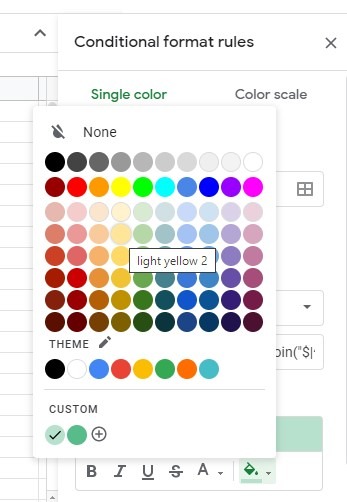
Finally, we should select the formatting style (in our case it will be a light yellow background for the cells that meet this condition).

Select ‘Done’ and the conditional formatting will be applied to the chosen range. Now you can easily see the smallest n values in each row in Google Sheets.

It wasn’t that hard, was it?

You can try it yourself by making a copy of the spreadsheet using the link attached below:

How to Highlight the Smallest N Values (Including 0) in Each Row in Google Sheets

Let’s begin setting your own conditional formatting to highlight the smallest n values in each row in Google Sheets, step-by-step.

1. First, you should select the range where you would like to apply conditional formatting. For this guide, I will choose the range B3:H12.

2. Then, go to the upper menu and select Format > Conditional Formatting. This will open the ‘Conditional format rules’ toolbar on the right.

3. Now, let’s go to the ‘Conditional format rules’ toolbar. In ‘Apply to range’, you will see the range you selected. Below that, you should set the rule. Click on the drop-down list below the ‘Format cells if…’ and choose ‘Custom formula is’.

4. Click on the ‘Value or formula’ field and start writing your formula. The formula should be written for one row and it will automatically be applied to the whole range. In our example, the formula to highlight the smallest n values in each row is =REGEXMATCH(B3&””, “^”&textjoin(“$|^”, 1, IFERROR(ARRAYFORMULA(
   SMALL($B3:$H3,sequence(1,3)))))&”$”).

5. Now you should select the formatting style you want to apply to the formatted cells. As you can see, you may change the font style and colour or the colour of the background. I will change the background colour to light yellow.

6. Finally, click on the ‘Done’ button below to close the toolbar and apply the conditional formatting rule you have set. As a result, the background colour of the cells with the smallest n values in each row will be light yellow now. If you followed the steps correctly, the cells that meet your criteria should now have the style you have chosen.

How to Highlight the Smallest N Values (Excluding 0) in Each Row in Google Sheets

If you want to highlight the smallest n values (excluding 0) in each row in Google Sheets, you should use this formula instead:

The only difference is the (filter($B3:$H3,$B3:$H3>0) part of the formula we added to filter 0 values.

When applying this conditional rule, all steps are the same. The only difference is the formula you write in the ‘Value or formula’ field.

That’s it, well done! You can now highlight the smallest n values (including and excluding 0) in each row in Google Sheets with conditional formatting. You can use it together with a wide range of other Google Sheets formulas to sort and filter your data according to your needs. 🙂

Get emails from us about Google Sheets.

Our goal this year is to create lots of rich, bite-sized tutorials for Google Sheets users like you. If you liked this one, you'll love what we are working on! Readers receive ✨ early access ✨ to new content.

Subscribe