How to Use FIND Function in Google Sheets

The FIND function in Google Sheets is useful if you want to return the position at which a string was found within the text.

The FIND function in Google Sheets is similar to the SEARCH function, with a slight difference. But will come to that later 🙂

Let’s take an example.

Say you have a text in the cell and need to know the exact position of the keyword or letter in the text.

So how do we do that?

Simple. The FIND function needs the string you’re looking for and the text to search within.

Optionally, if you’re not looking for the first concurrence of the string, you can add the character position at which the search starts. If you do not add the search position, the search will automatically start from the first character.

Let’s go straight into real examples where we will deal with actual values to better understand the FIND function in Google Sheets and see how you can write it yourself.

The Anatomy of the FIND Function

The syntax (the way we write) the FIND function is as follows:

=FIND(search_for, text_to_search, [starting_at])

Let’s break this down to understand the syntax of the FIND function and what each of these terms means:

• = the equal sign is how we begin any function in Google Sheets.
• FIND() is our function. We will have to add the string we want to search for, as well as the text to search within and a character position at which the search starts.
• search_for is the string you are looking for within text_to_search.
• text_to_search is the text within you are looking for the first concurrence of search_for.
• starting_at [optional, it is 1 by default] is the character position at which the search starts.

⚠️ A few notes you should know when writing your own FIND function in Google Sheets:

1. Unlike the SEARCH function, the FIND function is case sensitive, so you should pay attention to the uppercase and lowercase letters.
2. Wildcards (‘~’ tilde, ‘*’ asterisk, and ‘?’ question mark), used with certain Google Sheets functions to represent or replace a single or multiple other characters in functions, are not allowed with the FIND function.
3. The starting position is a number value that must be greater than or equal to 1 and less than or equal to the number of characters in the text you are searching within (text_to_search).
4. The FIND formula will return an error (#VALUE!) when the string you are searching for is not found within the text_to_search.

A Real Example of Using the FIND Function

Let’s take a look at the examples below to see how to use the FIND function in Google Sheets.

The first two formulas, in cells C2 and C3, are quite simple. The only difference is that you can either enter just the cell address or the text within you are looking for the first occurrence of the string. If you do not use the optional part of the syntax (starting_at) in the formula, it will count the text from the first character itself.

If you take a look at the third and fourth formulas, in cells C4 and C5, you will see that in the fourth formula (C5), we used the optional part of the syntax (starting_at), since there is the repetition of the same string “apple” twice. To find the position of the second concurrence of the string “apple”, we should first count the position of the first one, and in this case, that is #5 (as you can see in row 4). Now, we enter the first number higher than #5 and our search will start from there.

Finally, in the last formula, in cell C6, you can see that it returns an error (#VALUE!) since, unlike the SEARCH formula, the FIND formula in Google Sheets is case sensitive (meaning that uppercase and lowercase letters matter) 🙂

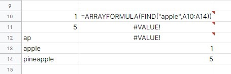
You can also use the FIND function to search the range of cells for the first occurrence of the string. To do this, you will need the ARRAYFORMULA wrapper. Your formula will now look like this

=ARRAYFORMULA(FIND(search_for, range, [starting_at])

If there is no string you are searching for, the formula will return an error (#VALUE!). But if the string is found, it will return the position of the string. Let’s see what happens if we try to search for the string “apple” within a range of five cells.

You can give it a try yourself by making a copy of the spreadsheet using the link below:

How to Use the FIND Function in Google Sheets

Let’s begin writing our own FIND function in Google Sheets, step-by-step.

1. First, click on any cell to make it active. You should click on the cell where you want to show your result. For this guide, I will be selecting B2.

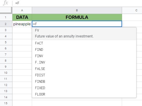
2. Then, type the equal sign ‘=’ to start off the function. After that, type the name of the function, which is ‘FIND’.

3. As you start to type the name of the function, you will see that the auto-suggested box with the names of the functions that start with ‘F’ will pop-up. You can close and ignore this pop-up, or you can select the FIND function by clicking on it, just make sure you click on the right one since sometimes more functions with similar names might be there.

4. After the opening bracket, you should add the string you are looking for. Make sure that search_for and text_to_search are not supplied in reverse order, or the formula will likely return an error (#VALUE!).

5. Enter a comma ‘,’ to act as a separator between the string you are looking for, and the text within you will perform the search.

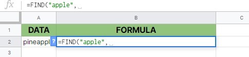
6. Once you have added the comma, enter the text within you will perform the search. You can also enter the cell address, no need to copy/paste the text.

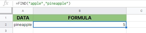
7. You can either close the function with the closing bracket ‘)‘ or hit your Enter key, which will close the bracket on the function and immediately output the result of the formula. If you followed my steps, the result in cell B2 would be 5 since this is the first position of the string “apple” within the selected text.

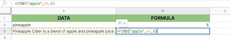
8. However, if you are not looking for the first concurrence of the string, and you would want to find the second position of the string “apple”, you should add the optional part of the syntax (starting_at). Enter a comma ‘,’ after the text within you will perform the search (or the cell address), and add the character position at which the search starts.

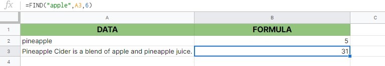
9. Close the function with the closing bracket ‘)‘ or hit your Enter key, and you will see that the result in cell B3 will be 31 since this is the second position of the string “apple” within the selected text.

That’s it! You did it! You can now use the FIND function together with the other Google Sheets formulas to create even more effective formulas that will help you with your work and save time 🙂

Get emails from us about Google Sheets.

Our goal this year is to create lots of rich, bite-sized tutorials for Google Sheets users like you. If you liked this one, you'll love what we are working on! Readers receive ✨ early access ✨ to new content. There will be no spam and you can unsubscribe at any time.

Subscribe