How to Use MATCH Function in Google Sheets

The MATCH function in Google Sheets is useful when you need to return the relative position of an item in a given range that matches an indicated value.

The MATCH function returns the position in an array rather than the value itself. This can be useful when determining the row or column associated with the matched value.

The Anatomy of the MATCH Function
A Real Example of Using MATCH Function
How to Use MATCH Function in Google Sheets

The rules for using the MATCH function in Google Sheets are as follows:

The function has two required arguments: the search key, and the range to search. The user can also indicate how to search as a third argument
The function then outputs an integer corresponding to the relative position of an item in a range.

Let’s look into a quick use case where we can use the MATCH function.

Suppose you have a business selling office supplies. You have a spreadsheet table of products sorted by the total number of orders they’ve received in the past year. The items are sorted in descending order, where the product in the first row will be the most-ordered item.

Given a specific product name or product ID, how can we determine which row they appear in our table?

We can find the relative position easily using the MATCH function. After finding the relative position, we can then use other functions like INDEX to retrieve information in the same row.

Now that we know when to use the MATCH function, let’s see how it can be used on an actual spreadsheet.

The Anatomy of the MATCH Function

The syntax of the MATCH function is as follows:

=MATCH(search_key, range, [search_type])

Let’s look at each term to understand what they mean.

‘=’ the equal sign is how we start any function in Google Sheets.
MATCH() is our MATCH function. The function returns the relative position of a matching item in a range.
search_key refers to the value you want to find a match for.
range refers to the one-dimensional array to be searched.
search_type refers to the method to use for searching. ‘1’ indicates that the range is sorted in ascending order, and you want to return the largest value less than or equal to the search key. ‘0’ indicates that you want an exact match. ‘-1’ is similar to ‘1’ but assumes that the range is in descending order.

A Real Example of Using MATCH Function

Let’s take a look at a real example of the MATCH function being used in a Google Sheets spreadsheet.

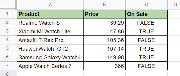
The table below includes a list of smartwatch products and their corresponding prices. We have ordered each entry by price in ascending order. Using the MATCH function, we can search for a particular smartwatch and see what position it can be found on the table.

MATCH function in Google Sheets

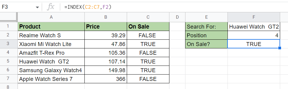
In addition to the position, we’ve also used the result of our MATCH function to retrieve the corresponding value in the ‘On Sale’ column.

To get the position in cell F2, we will need to use the following formula:

=MATCH(F1,A2:A7,0)

Let’s try to understand how this formula works. The first argument for the MATCH function determines the string to try to match with. In this case, we’ll reference cell F1 in our spreadsheet.

Next, we’ll need to specify which range to search in. Since our search string refers to the product name, we’ll need to search for the string in the range A2:A7. The last argument specifies that we want to look for an exact match rather than an approximate match.

You can make your own copy of the spreadsheet above using the link attached below.

Make a copy of example spreadsheet

If you’re ready to try out the MATCH function in Google Sheets, let’s begin writing it ourselves!

How to Use MATCH Function in Google Sheets

This section will guide you through each step needed to start using the MATCH function in Google Sheets. You’ll learn how we can use the MATCH function to get the position of a certain value in a one-dimensional array. The range could either be a horizontal or vertical array.

Follow these steps to start using the MATCH function:

First, determine the field you want to search in. In this example, we want to find a match based on the product column. Since the order of each entry is important, ensure that you already have a sorted table.
Next, we’ll specify two additional cells in our spreadsheet. The first cell will be where the user will type in the search string. The second cell will hold our MATCH function.
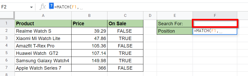
Type “=MATCH(“ in your spreadsheet to begin the MATCH function. You may find a tooltip box with hints on how to use the MATCH function. We can click on the arrow on the top-right-hand corner of the box to minimize it if necessary.
Next, select cell F1 as the first argument.
For the second argument, add a reference to the cell range you want to find a match in. In this example, we’ll use the range A2:A7.
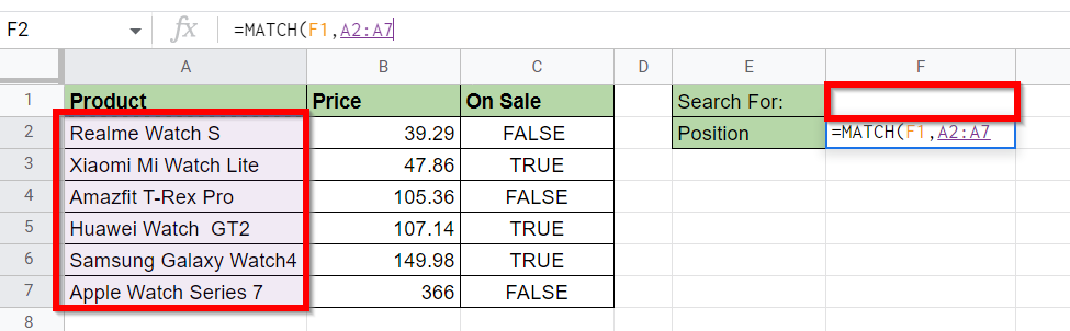
For the last argument, type ‘0’ to indicate that you want an exact match.
Your formula should now return the relative position given a product name.
We can expand on the results by using the INDEX function to get values in the same row. In the INDEX function below, we used the result of our MATCH function to get another value in that same row.

This step-by-step guide should be all you need to start using the MATCH function in Google Sheets. Our guide shows how this function can return the relative position of a value in a range.

Overall, the MATCH function is just one of many useful data functions in Google Sheets. With so many other Google Sheets functions available, you can surely find one that suits your use case.

Are you interested in learning more about what Google Sheets can do? Subscribe to our newsletter to find out about the latest Google Sheets guides and tutorials from us.