How to Use Query With Importrange in Google Sheets

The Query with Importrange in Google Sheets is useful if you want to pull the exact data that you need.

The Query with Importrange does this by merely using the QUERY function first, then nest the  IMPORTRANGE function in the formula.

To break it down into its two components:

The QUERY function is one of the most versatile functions in Google Sheets. With QUERY, you can do actions like lookup, sum, count, average, filter, and sort.

On the other hand, the IMPORTRANGE function allows you to import and transfer a range of cells from one spreadsheet to another.

Let’s take an example.

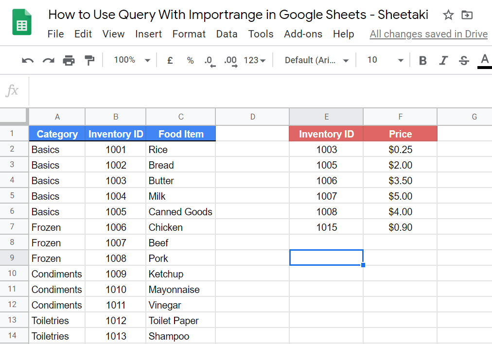
Say, I own a supermarket with hundreds of products. I currently maintain two spreadsheets, one main spreadsheet for all the inventory information — ‘Category’, ‘Inventory ID’, and ‘Food Item’. Whereas, the other spreadsheet contains — ‘Inventory ID’, ‘Quantity’, ‘Price’, and ‘Value’.

I want to import the Inventory ID and the price of items whose quantity is already less than 10, to our main spreadsheet.

So how do we do that?

Easy. We can use our QUERY with IMPORTRANGE to import only the Inventory ID and price to our main spreadsheet. We will supply the functions with the right attributes.

Ultimately, the functions will output a list of Inventory ID and Price of items whose inventory count is less than 10.

You can do a lot of things with the QUERY with IMPORTRANGE functions. In fact, you can import multiple spreadsheets, provided that you have specified all your criteria.

It is one of the many powerful tools to have in your arsenal to solve a lot of your business data entry problems and save half of your data entry time.

Let’s go straight into real-business examples where we deal with actual values and textual strings and how we can write our own Query with Importrange function in Google Sheets.

The Anatomy of the Query with Importrange Function

So the syntax (or how we write) the Query with Importrange function is as follows:

=QUERY(IMPORTRANGE(spreadsheet_url, range_string), query, [headers])

Here’s what each of those terminologies mean:

• = we must add the equal sign to start off any function in Google Sheets
• QUERY() is the function responsible for selecting what ranges to display based on your criteria
• IMPORTRANGE() is a function that allows you to import values from cell ranges in another spreadsheet into your own spreadsheet
• spreadsheet_url is the link to the spreadsheet where the desired cells are coming from
• range_string defines the range of cells to be imported. Usually, this has two components: the name of the sheet and the cells range. The components are separated by an exclamation point (!) and enclosed in a quote-unquote symbol, (” “). For example, “Data!A2:D16”
• query includes the criteria or condition
• [headers] are optional. But, you usually put “1” if the spreadsheet consists of a row of headers.

Now, it may look complicated but, rest assured that we will go through the step-by-step process on how to exactly use the Query with Importrange functions in Google Sheets. 🙂

A Real Example of Using Query with Importrange Function

Have a look at the example below to see how Query with Importrange functions is used in Google Sheets.

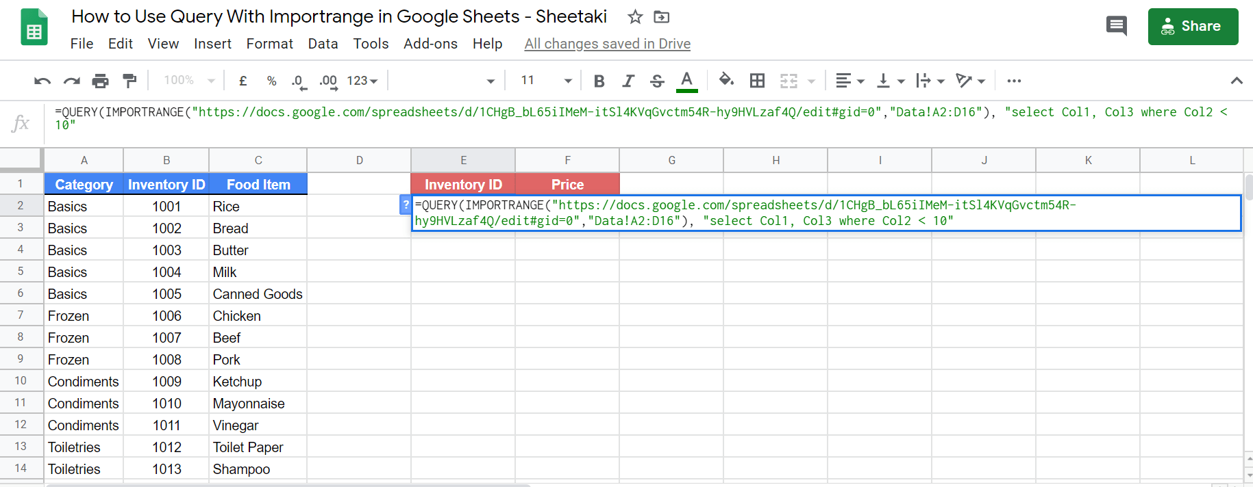
As you can see in the images above, we have two spreadsheets, and the Query with Importrange functions is used to import the ‘Inventory ID’ and ‘Price’ from Spreadsheet 2 to Spreadsheet 1. The function is as follows:

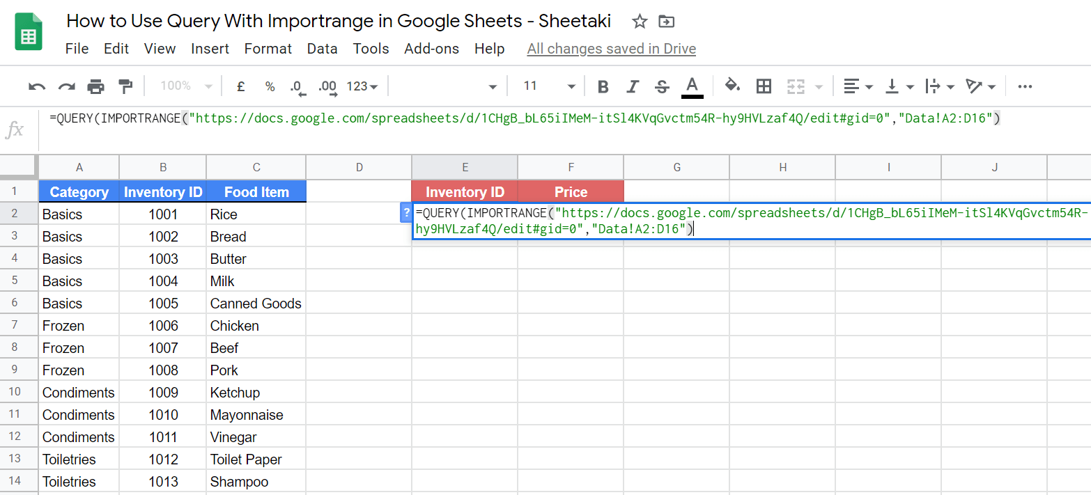
=QUERY(IMPORTRANGE("https://docs.google.com/spreadsheets/d/1CHgB_bL65iIMeM-itSl4KVqGvctm54R-hy9HVLzaf4Q/edit#gid=0","Data!A2:D16"), "select Col1,Col3 where Col2 < 10")

Here’s what this example does:

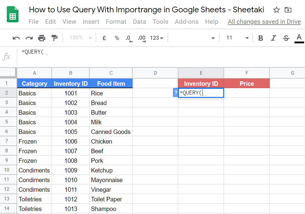
• We have actively selected the cell under E1, and we want to use the Query with Importrange function to import Inventory ID and Price of items whose quantity is already less than 10.
• As you can see in the images above, the Inventory ID and Price of items are found in the 2nd spreadsheet. So, basically, we want to import that information from Spreadsheet 2 to our main spreadsheet.
• We started with the Query function and had the Importrange nested. We supplied the right attributes for each function.
• As a condition, we used less than (<) as our comparison operator.
• Our function outputs only the Inventory ID and Price of items that have an inventory count of less than 10.

Easy, right?

You may try the examples out yourself using the links I have attached below:

Let’s begin writing our own Query with Importrange function in Google Sheets.

How to Use Query with Importrange Function in Google Sheets

1. Prepare your spreadsheets. Make sure you have at least two spreadsheets to make the Query with Importrange Function work seamlessly.

2. Great! Now click on any cell to make it active. This is where you want to put your formula and where you want your data to be imported. For this guide, I have selected the cell E2 from my first spreadsheet.

3. Start your formula with the QUERY function and an open parenthesis “(“.

4. Next, write the IMPORTRANGE function and follow it up with an open parenthesis “(“.

5. Enclosed in a quote-unquote symbol (” “), paste the URL or link of the other spreadsheet where the data you want to import is from. Then, add a comma to separate it from the next attribute.

6. Great! Now, let’s add the range_string. Write the name of the spreadsheet where your desired data will be imported from, then followed by the cell range. For this guide, I have named the spreadsheet as Data, and my cell range is A2:D16. Then close the string with a close parenthesis “)“.

7. We are now ready to add the condition. We want to import the ‘Inventory ID’ and the ‘Price’ which is in columns 1 and 3 (or columns A and C), provided that it meets our criteria, “where column 2 or the Quantity is less than 10“. Therefore, our condition would be select Col1, Col3 where Col2 < 10.

8. Close our formula with a close parenthesis, “)“, then hit on the Enter key.

Great job! 👏 That’s pretty much it.

You can now use the QUERY with IMPORTRANGE in Google Sheets together with the other numerous Google Sheets formulas to create even more effective formulas. 🙂

Get emails from us about Google Sheets.

Our goal this year is to create lots of rich, bite-sized tutorials for Google Sheets users like you. If you liked this one, you'll love what we are working on! Readers receive ✨ early access ✨ to new content. There will be no spam and you can unsubscribe at any time.

Subscribe