How to Share Specific Tabs in Google Sheets

Learning to share specific tabs in Google Sheets may come in useful when you want to share a link on the specific tab in Google Sheets or even only sharing one tab without giving viewers access to other tabs in Google Sheets.

Google Sheets can be seamlessly shared among several people to promote collaborations in a working environment. 

However, in certain situations, you only want to share specific Google Sheets tabs without giving access to the other tabs. We are here to teach you how! 🎉

Share Specific Tabs in Google Sheets to Other User

Very often, one Google Sheets would contain many tabs containing important information. However, you need to share the Google Sheets with our colleague to input data into a certain tab only. 

In these situations, you are worried if she would accidentally edit the other tabs causing a mess.

By using an example, we would demonstrate how to share access to only a specific tab in Google Sheet to avoid such incidents.

Example 1

For example, your Google Sheets contain sales achieved during the year. As March has recently ended, you would like your colleague to fill in the recorded sales for each outlet.

Knowing that the sales recorded for January and February are finalized, you do not wish any adjustments are made to those tabs. 

Follow the steps below to learn how only to share a specific tab!

1. First, click on the tab that we do not wish to share access to.  

2. Then we will click on the arrow button. This would cause a list of options to appear. We would then click on Protect sheet.

3. A sidebar would then appear on the right side of your screen. Press Set permissions.

4. A pop-up will appear. We can now restrict who can edit the particular tab. This would prevent other people from editing it. They would need your permission to edit the protected tab.

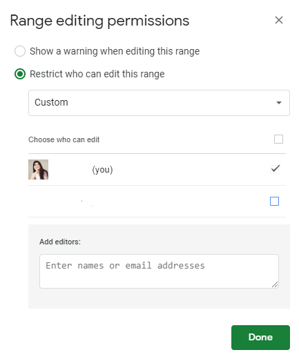
5. A “locked” symbol would appear next to your tab name once you press Done.

As a result, your colleague would only be able to edit the “March” tab. If she tries to edit the other tabs, a pop-up would appear to instruct them to contact you for permission. 

Share Specific Tabs in Google Sheets Using IMPORTRANGE Function

In some situations, the Google Sheet that you would like to share may have too many tabs. This would make protecting all tabs tedious and time-consuming.

In such circumstances, we would suggest using the IMPORTRANGE function to import the range of cells from a specified tab to a new Google Sheets spread.

Let us explain how does the IMPORTRANGE function work.  

The way we write the IMPORTRANGE function is: 

= IMPORTRANGE(spreadsheet_url, range_string)

Let us help you understand the context of the function:

• The equal sign =  is how we start any function in Google Sheets.
• IMPORTRANGE() is our function. To make it work correctly, we need to add two attributes, namely the spreadsheet_url and range_string. 
• The spreadsheet_url is the URL of the spreadsheet from where data will be imported from.
• The range_string is a string that contains the tab name and the specified range.

Let us use an example to demonstrate how to utilize the IMPORTRANGE function to only share a specified tab in Google Sheets.

Do take note that by using the IMPORTRANGE function, viewers can see the URL link used in the formula. Hence, we need to restrict the access for the master Google Sheets spread.

Example 1

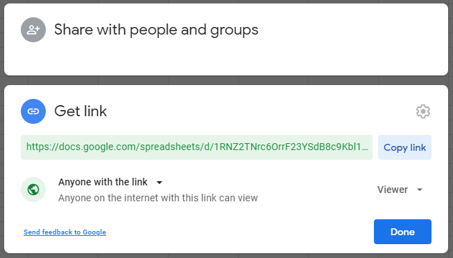
1. First, we need to restrict the access for the master Google Sheets spread. On the top right corner, click on the Share button.

2. Then, a pop-up would appear. We would change ‘Anyone with the link‘ to ‘Restricted‘. This would prevent viewers from copying the URL and getting access. 

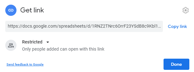
3. Once we are done with restricting the access of the Google Sheets to only those who are manually added, we need to copy the link provided within the pop-up. This would be the URL used in the IMPORTRANGE function in the new Google Sheets spread.

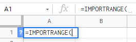
4. In the new Google Sheets spread, select the cell you would like to input the formula in. In this example, it would be A1. Then, insert an equal sign = and insert the function name IMPORTRANGE.

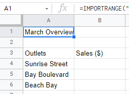
5. We would then insert the URL of the specified tab in the master Google Sheets spread that we want to share. Remember to insert opening and closing quotation marks"".

6. Next, we will specify the desired tab name and range to be shown. In our case, it would be “March!B2:C7”. Once you hit enter, the formula would return a #REF! error. Click on the cell and press Allow access to allow access to the master spread.

7. Your input would look like this once access is allowed. As you can see, the function only imports the data within the range specified but not the formats. You can format the data to your desired preference.

Using the IMPORTRANGE function also helps to hide all the other tabs within the master Google Sheets spread as they do not have permission to view it at all.

You may make a copy of the spreadsheet using the link attached below and try it for yourself:

There you go! These are two simple yet effective ways to share specific tabs in Google Sheets to avoid possible alterations to your original tabs!

Get emails from us about Google Sheets.

Our goal this year is to create lots of rich, bite-sized tutorials for Google Sheets users like you. If you liked this one, you'll love what we are working on! Readers receive ✨ early access ✨ to new content.

Subscribe