How to Expand Dates and Assign Values in Google Sheets

To expand dates and assign values in Google Sheets is useful if you have a schedule, and you want to assign a specific value at a given date which is between two dates of the schedule.

We will combine two functions and wrap them in a QUERY function to accomplish this. We can use the SEQUENCE function to expand dates and the VLOOKUP function to assign values.

Let’s define the task and the expected output first:

• We have ranges of dates in our data set, and each range has a value that we would like to assign to an expanded list of each date of these ranges.

We are referring to days as dates here. Each day in the ranges should appear in the expanded list, and their assigned value should be put next to these days.

Let’s visualize our expected output.

 

Here we have an input table with the date ranges (in cells E2:F5) and cities assigned to these dates (in cells G2:G5). The output we will create can be seen in cells A1:B21. The task is to have a separate cell for each day in the defined ranges and to put the assigned city names next to the cells of the days.

For example, a frequent traveller might want to have such a list with his travelling days and the destinations.

 

⚠️ Ground Rules Before Starting to Work with This Example

1. Each date range has an assigned value, none of them is blank.
2. The date ranges all have a start and end date.
3. The date ranges don’t overlap, so each day is included in only one date range. (From our example: the traveller will not travel to more than one city in one day)
4. But we allow non-connecting date ranges, so there can be days missing in between the date ranges that should not be included in the final list. (From our example: the days when the traveller stays at home)

 

 

How to Expand Dates Using SEQUENCE Step by Step in Google Sheets

First, we want to expand the dates of our ranges. In other words, to auto-populate the dates. We are using the SEQUENCE function to do this.

The syntax of the SEQUENCE function is the following:

=SEQUENCE (rows, columns, start, step)

Let’s dissect this thing and learn about each of these terms:

• = the equal sign is just how we begin any function in Google Sheets.
• SEQUENCE this is our function. We will have to add the corresponding value(s) into it for it to work.
• rows is a required field that represents the number of rows to return.
• columns is an optional field that represents the number of columns to return. If you omit using it, the returned array will have one column.
• start is an optional field that represents the number to start the sequence at. If you ignore using it, the sequence will start at 1.
• step is an optional field that represents the amount to increase (or decrease) each number in the sequence. By default, it will increase the sequence by 1.

The number of rows is exactly what we would like to create an expression for. We need to calculate how many days are in between the date ranges of the example.

---

Step 1: Find the Smallest and Largest Values of the Range

The first step to calculate this is to find the earliest and latest date in the range E2:F5. We can use the simplest MIN and MAX functions to get these dates and find the smallest and the largest dates of the ranges.

To get the earliest day of all the ranges, we will write:

=MIN(E2:F5)

And to get the latest day we will write the same, but with the MAX function:

=MAX(E2:F5)

---

Step 2: Expand the Dates with the SEQUENCE function

Next, we will put these expressions into the SEQUENCE function.

We calculate the number of days between the latest (maximum) and earliest (minimum) dates. And since we want to include these bordering dates as well, we have to add 1 to this calculation.

We also want to define the starting value in the expanded list and write it as the third argument of the above-described SEQUENCE syntax. It should be the first day of the earliest range so that the start argument will be the smallest date in the data set.

So we defined the rows and the start arguments. We are good with the default values for the other two arguments. However, as you can see below, we need to explicitly write the second argument (column = 1) to be able to define the third argument.

The whole formula will look like this:

=SEQUENCE(days(MAX(E2:F5), MIN(E2:F5))+1,1, MIN(E2:F5))

When you enter this formula in the cell A2, you will get a column of numbers instead of dates, but don’t worry, it is fine. To format the values to proper date format, you have to go to the menu Format > Number and then click on ‘Date’.

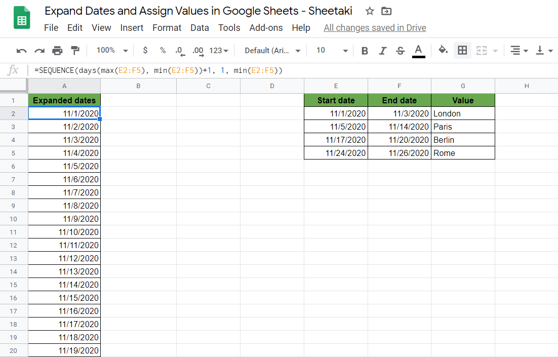
Great, now we have all the days between the minimum and maximum dates of our date ranges.

The problem is that we have some extra days here that are not included in any of our start and end date ranges. For example, none of the original ranges has the days 11/4/2020 or 11/15/2020. We have to filter out the unwanted dates, but we will get back to this issue later.

---

Step 3: Define the Start and End Dates of Each Value

The next step is to create a helper table to later assign the values to the days.

We copy each start date to a separate column and also the city names to the next column. After each start date in the helper table, we will insert a new row that has the respective date range’s end date + 1 day. Next to these dates, we will not put any city names but leave those cells blank.

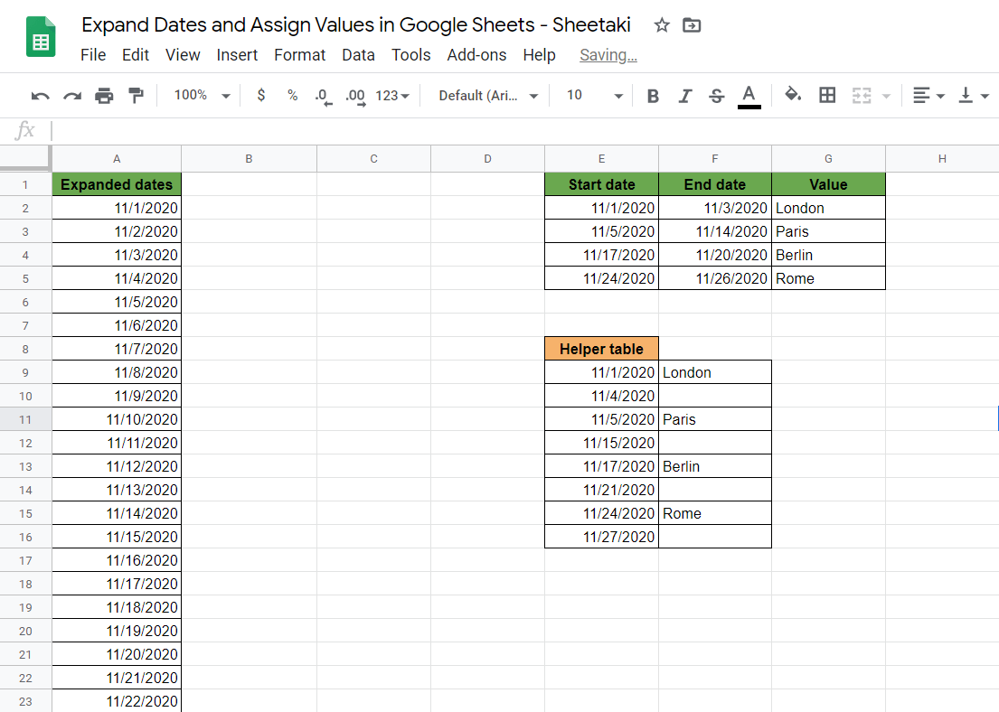
This way, we guarantee that we defined where each date range ends and starting from which day it should not be assigned the city of the previous date range.

 

 

How to Assign Values Using VLOOKUP in Google Sheets

We are using the powerful VLOOKUP function of Google Sheets to assign values to the expanded dates. VLOOKUP means vertically lookup for some value (search key) in our data set.

The syntax of the VLOOKUPfunction is:

=VLOOKUP(search_key, range, index, is_sorted)

Let’s dissect this as well and understand what each of these terms means:

• = the equal sign is just how we start any function in Google Sheets.
• VLOOKUP this is our function. We will have to add the corresponding value(s) into it for it to work.
• search_key(s) are the values we want to lookup.
• range is where the lookup value is located.
• index describes which column of the range are we using as values.
• is_sorted is an optional argument. It’s 1 (true) by default meaning an approximate match (the nearest match is returned). If you want an exact match, you can set it false.

---

Step 1: Use the Expanded List of Dates in a VLOOKUP function

Now let’s see how we should use this function in our example.

• The search_key will be the expanded list of dates because we want to lookup for these values.
• The range should describe which value is assigned to which dates, so we should use our helper table here to define the start and end date for each city.
• Th index will be 2, since we want to use the cities as return values and they are in the second column of the range.
• We don’t need the is_sorted argument here, because it makes no difference with text values.

The VLOOKUPfunction to assign values is:

=VLOOKUP(A2:A,E9:F,2,1)

If we write this is the first cell of the column of the assigned values (B2 in the example), it works because we get London as a result.

---

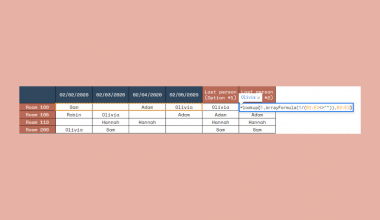
Step 2: Use ArrayFormula to Repeat the Task on the Whole Data Set

We could repeat the previous expression in each cell of column B to assign the cities, but there is a simpler and more elegant solution.

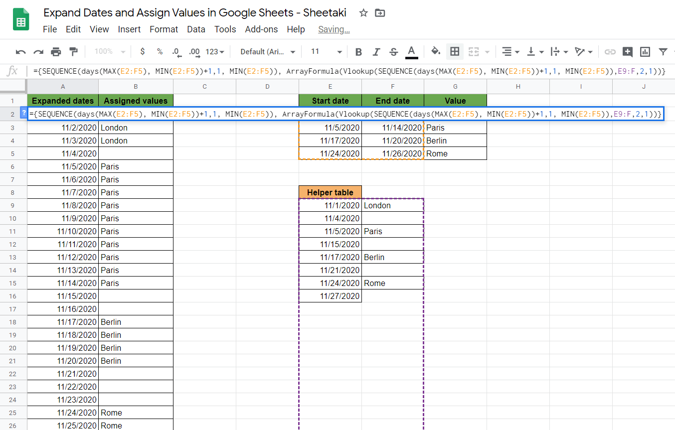
We are using an ArrayFormula to execute the function not only in one cell but in the whole array of dates at once.

=ArrayFormula(VLOOKUP(A2:A,E9:F,2,1))

This way, we don’t have to write the same expression in every cell of column B, but only in the first cell, and it will be performed on the whole array of dates.

The result can be seen in this picture:

 

 

How to Do All This in One Formula and Filter Out Unwanted Rows Using QUERY

We might want to combine the SEQUENCE and VLOOKUP functions in one single formula to automate the whole table even more.

Also, we still don’t have our expected result presented at the beginning, because there are extra rows in it.

---

Step 1: Use the Previous Two Functions in One Array

Let’s use our previous two functions together in an array. We do this by putting two expressions into {} brackets, separated by a comma. First, we insert the SEQUENCE function and then the VLOOKUP function in the ArrayFormula.

={SEQUENCE(days(MAX(E2:F5), MIN(E2:F5))+1,1, MIN(E2:F5)), ArrayFormula(VLOOKUP(A2:A,E9:F,2,1))}

---

Step 2: Replace the Expanded Dates Cells with Its SEQUENCE Formula

The VLOOKUP formula is using the results of the first SEQUENCE formula as its search_key, so we can also replace the first argument of the VLOOKUP function with the SEQUENCE formula.

={SEQUENCE(days(MAX(E2:F5), MIN(E2:F5))+1,1, MIN(E2:F5)), ArrayFormula(VLOOKUP(SEQUENCE(days(MAX(E2:F5), MIN(E2:F5))+1,1, MIN(E2:F5)),E9:F,2,1))}

---

Step 3: Remove Empty Values Using QUERY

Now is the moment to filter out the rows without an assigned value. As you can see, there are many rows without an assigned city name. The solution to this is a bit more complicated, as it involves writing a QUERY function.

We will use a query to remove the rows without an assigned value (without a city) in the second column.

Although this function is a bit more advanced, the syntax of the QUERY function is very similar to other functions:

=QUERY(data, query, headers)

Let’s understand what each of these terms means:

• = the equal sign is just how we start any function in Google Sheets.
• QUERY this is our function. We will have to add the corresponding value(s) into it for it to work.
• data is the range of cells to perform the query on.
• query is the query to perform, written in the query language of Google Sheets.
• headers are optional, and it means the number of header rows at the top of data.

The data is all of the previous result set we just calculated above. We will put our result cell range here.

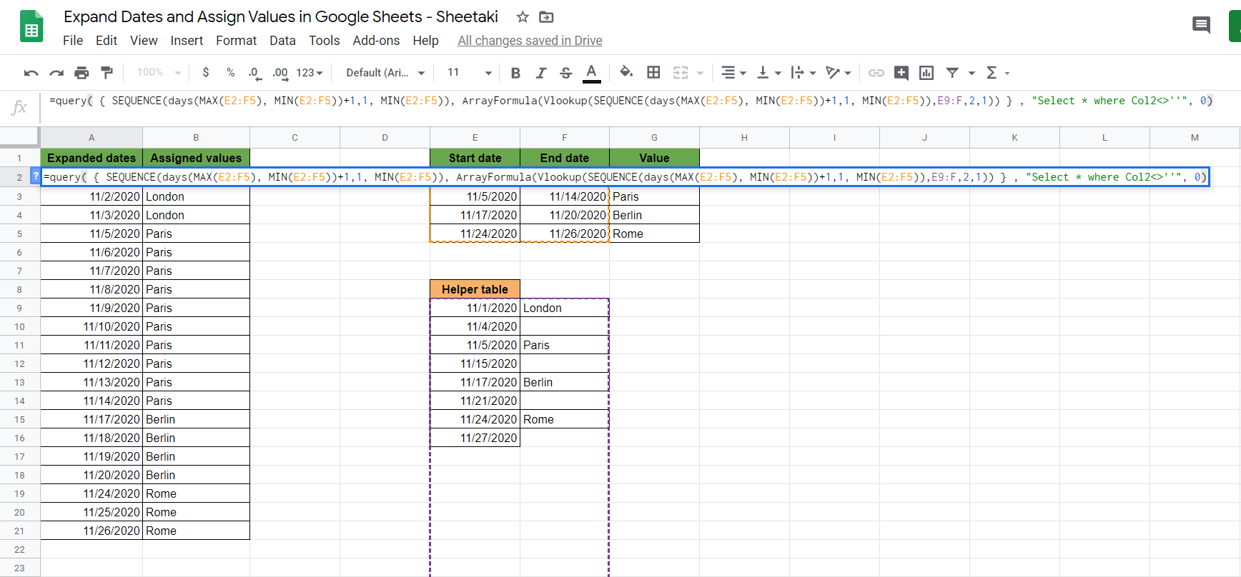
The query part should be written in an SQL-like search query expression. We want to keep the rows where the assigned value (the second column) exist, in other words, where it is NOT blank. The following expression will do this: “Select * where Col2<>”.

Therefore, the whole QUERY function will look like this:

=QUERY( { our previous formula } , "Select * where Col2<>''", 0)

Let’s replace “our previous formula” with the actual formula:

=QUERY({SEQUENCE(days(MAX(E2:F5), MIN(E2:F5))+1,1, MIN(E2:F5)), ArrayFormula(VLOOKUP(SEQUENCE(days(MAX(E2:F5), MIN(E2:F5))+1,1, MIN(E2:F5)),E9:F,2,1))}, "Select * where Col2<>''", 0)

We just have to write this combined formula in cell A2 and hit Enter. As a result, we have a perfect list with the expanded dates and their assigned values.

 

That’s it! This is how you expand dates and assign values in Google Sheets using the SEQUENCE, VLOOKUP and QUERY functions. 👏🏆

Feel free to make a copy of the spreadsheet using the link I have attached below and try it for yourself:

You can now expand dates and assign values together with the other numerous Google Sheets formulas to create even useful powerful. 🙂