The ACCRINT function in Google Sheets is designed specifically to calculate the accrued interest for an investment or a loan; whether this interest is paid annually, semi-annually, or quarterly.
Notice that the function’s name (ACCRINT) is driven from “Accrued Interest”.
Table of Contents
This function calculates the supposed value of a deposit or a loan, after some time.
So, what’s accrued interest?
In simple form, accrued interest is the accumulated interest on a principal value over a time period. Let’s see an example to understand the concept more.
Say you decided to take a student loan to get through college, you took $10,000. The interest rate was 10%. What would be the accrued interest after 4 years?
Well, here’s how it’s calculated.
Accrued Interest = Principal value x Rate365 x time period
So, Accrued Interest = $10,000 x 0.1365 x 365 x 4 = $4,000
Which means that after 4 years you owe the bank $10,000 + $4,000 = $14,000
This is the idea of accrued interest in its simplest form, there are some more details though, let’s go ahead and find out more.
The Anatomy of the ACCRINT Function in Google Sheets
So, the ACCRINT function shall be written as follows:
=ACCRINT(issue, first payment, settlement, rate, redemption, frequency, day count convention)
Let’s dissect this thing and understand what each of these terms means:
- = (the equal sign) is just how we start any function in Google Sheets.
ACCRINTis the name of the function we are using.- () These parentheses are used to host the two values we put in our function, and a comma “,” must separate these values.
Note that the values hosted in any google sheets function are called arguments.
- (issue) The date the security was initially issued.
- (first payment) The first date interest will be paid.
- (settlement) The settlement date of the security, the date after issuance when the security is delivered to the buyer.
- (rate) The annualized rate of interest.
- (redemption) The loaned or invested amount (the original value to be redeemed).
- (frequency) The number of payments per year. This argument takes either 1, 2 or 4; 1 for annual, 2 for once every six months and 3 for once every three months.
- (day count convention) Final argument. An indicator of what day count method to use.
Know that the final argument is optional, and it takes from 0 to 4, and its default value is 0; 0 for 30/360, 1 for actual/actual, 2 for actual/360, 3 for actual/365, or 4 for 30/360 European.
Notice that if any of the first 6 arguments weren’t specified correctly, the function would result in an error.
So, before we go deeper in to the function, there are a few things to be aware of in the ACCRINT function, otherwise you will get an error:
- The issue date must be less than or equal to the settlement date (issue date ≤ settlement date).
- The frequency (6th argument) must be between these 3 numbers; 1,2 and 4.
- The day count conversion (7th argument) must be from 0 to 4 inclusive.
Now for further explanation, let’s go through the ACCRINT function together, and you will understand it once you start practicing its application.
A Real Example of Using ACCRINT Function
Take a look at the example below to see how the ACCRINT function is used in Google Sheets.
- Issue date = 1-Jan-2020
- First payment date = 1-Aug-2020
- Settlement date = 1-Jul-2021
- Interest rate = 0.1
- Redemption = $1000
- Frequency = 4
- Day count convention = 2
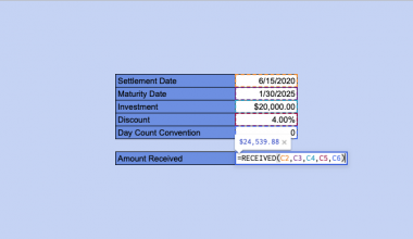
And that’s how we write these data in google sheets.
As you can see in the table, the ACCRINT Formula row has the formula of the ACCRINT function, and the ACCRINT Result column has the formula’s result.
Now let’s look closely at the formula we have.
=ACCRINT (B2, B3, B4, B5, B6, B7, B8)
Or
=ACCRINT (1/1/2020, 8/1/2020, 7/1/2021, 0.1, 1000, 4, 2)
You may make a copy of the spreadsheet using the link attached below.
Make a copy of example spreadsheet
For those who are curious about the core of this formula. Here’s how this function works. See the following example, where we are given these details:
Here’s the equation being calculated in the background.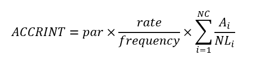
Where:
- par = redemption value
- NC = number of periods where interest is added that fit in the odd period (Fractions are raid to the next whole number).
- Ai = number of the accrued days for the ith interest period within the odd period.
- NLi = normal length in days of the interest period within the odd period.
Obviously, you don’t have to 100% understand the formula of the ACCRINT function. After all, Google Sheets is here to take care of the complicated calculations for you.
How to Use the ACCRINT Function in Google Sheets
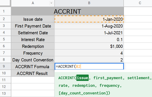
- Simply click on any cell to make it the active cell. For this guide, I will be selecting B9, where I want to show my formula. Then type ‘=‘.
- Now, type ‘ACC‘ and click on the
ACCRINTfunction or press Tab to select it.
Notice that there are two options to select from, we are only concerned with the ACCRINT function now, so don’t confuse it with the other one that ends with an “M”.
- Now, fill in the first argument of the function; issue, which would be the value in cell B2. So, you can select it or type ‘B2‘.
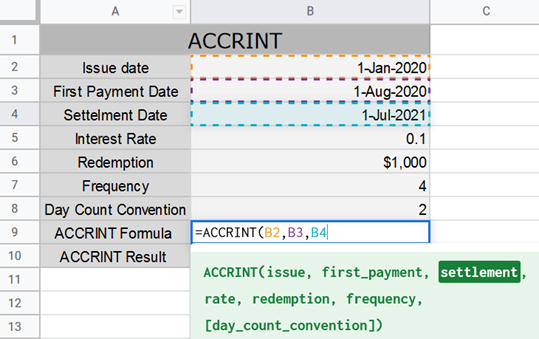
- Then, type comma ‘,‘.
- Now go ahead and select the second argument; first_payment, which is the value in B3.

- Then, type comma ‘,‘ and select the third argument; settlement, which would be the date in cell B4.
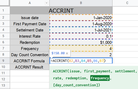
- Type comma ‘,á and select the forth argument; rate, which would be the date in cell B5.

- Now after you type another comma, put in the fifth argument; redemption, which would be in B6.

- For the 6th argument; frequency, we put the value in B7.
- Finally, for the 7th argument; [day_count_convention], we put in B8, close the parenthesis and press Enter.
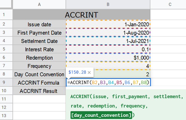
Notice that the result was already calculated without the final argument of the function, since it’s optional. We still can’t ignore the 7th argument, because it makes a difference, precisely $0.28 in our case.
That’s pretty much it. Congrats! You now learned the ACCRINT function in Google Sheets.
Are you thirsty for more knowledge about some more efficient Google Sheets functions? Well, lucky for you, you’re one click away from your destination.