The DOLLARFR function in Google Sheets is useful if you want to convert a price given as a decimal value into a decimal fraction, which is used in securities denominated in dollars.
Meaning, it converts a decimal number to its equivalent in fractional numbers. The DOLLARFR is mostly used by Financial Analysts who deal with financial reports and stock market quotes.
Table of Contents
The rules for using DOLLARFR function in Google Sheets are as follows:
- The DOLLARFR function is for visual only. Value it returns can’t be used in other calculations or in charts.
- The DOLLARFR can also be used to convert non-dollar data.
Let’s take an example.
My previous manager asked me to create a report that shows the length of service of each of his subordinates. The given data is as follows:
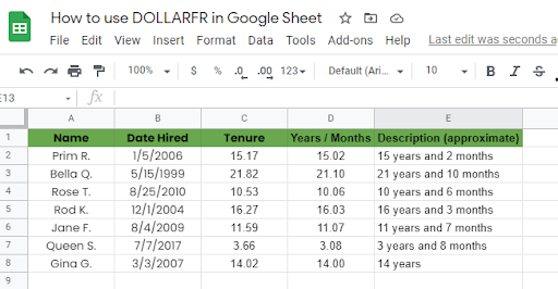
He asked me explicitly to calculate how long, in terms of years and months, each of them has been working for the company from today.
I was able to come up with the values 15.17 years, 21.82 years, and so on and so forth in column C. However, the decimal numbers on these values (i.e .17 and .82) don’t mean the exact numbers in months.
That’s where we can use the DOLLARFR function. We can convert these numbers in a way that it reads as X number of years and Y number of months. See column D and column E for the description.
Let’s have another example!
John needs to report to his manager the average time, in hours and minutes, the entire team has performed for a specific task. He managed to be able to come up with the average, however, it is in decimal format.
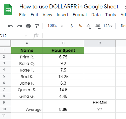
He’s sure that the average is at 8 hours, but .86 doesn’t mean it is the minute part that he’s looking for.
John here can use the DOLLARFR function to be able to convert the 8.86 value in a way that reads as 8 hours and 52 minutes.
There are many ways that these example cases can be solved. DOLLARFR can surely be one of them if you’re looking for a quick solution. 🙂
Watch out for a more advanced tutorial and examples on how you can use DOLLARFR functions in the coming weeks. Be sure to subscribe to be notified.
Awesome! Let’s begin getting to know more about our DOLLARFR function in Google Sheets.
The Anatomy of the DOLLARFR Function
So the syntax (the way we write) the DOLLARFR function is as follows:
=DOLLARFR(decimal_price, unit)
Let’s dissect this thing and understand what each of these terms means:
- = the equal sign is just how we start any function in Google Sheets. It is how Google sheets understand that we are asking it to either do a computation or use a function.
- DOLLARFR() this is our DOLLARFR function. DOLLARFR converts the decimal part of the “decimal_price” number into a fraction with the denominator being “unit.”
- decimal_price is the first argument that is a decimal number, given as price quotation
- unit is the second argument that is the integer (example 4 for 1/4ths, 8 for 1/8ths, or 32 for 1/32nds) to use in the denominator (divisor) of a fraction. It must be an integer. But if the decimal value is used, Google Sheet will truncate it to an integer.
A Real Example of Using DOLLARFR Function
Take a look at the example below to see how DOLLARFR functions are used in Google Sheets.

As you can see, the DOLLARFR only changes the decimal part of the given decimal price in Column A. The integer remained unchanged even after converted by the DOLLARFR function.
Take a look at the example in cell A2, DOLLARFR function converts the decimal number 2.25 to a number that reads as 2 and 1/4 in cell C2. It means that the 0.25 in A2 is the same as 1/4, while the 2 remained the same.
For decimal price in cell A3, the function converts the number 3.5 to a number that reads as 3 and 4/8 or simply 1/2, while the whole number (3) remains as is.
You may make a copy of the spreadsheet using the link I have attached below.
How to Use DOLLARFR Function in Google Sheets
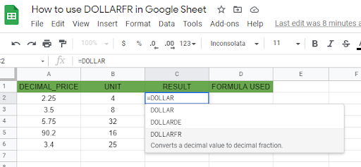
- Simply click on any cell to make it the active cell. For this guide, I will be selecting C2 where I want to show my result.

- Next, type the equal sign ‘=‘ to begin the function and then followed by the name of the function, which is our ‘dollar‘ (or ‘DOLLAR‘, not case sensitive).
- You should find that the auto-suggest box appears with the names of the functions that all start with DOLLAR. You may use your mouse to click on the DOLLARFR or use your down arrow keys to highlight and hit the enter key. Alternatively, you may completely type DOLLARFR and hit Tab to let you use that function.
- Now the fun part! Let’s give our function the first argument, which is the decimal_price. You may pass a constant data by typing the exact decimal after the parenthesis.

- To let the Google sheet know that we’re done typing our first argument, we should now type in the delimiter or the character that separates each argument on a function. In this case, type comma(,) followed by the second argument, which is the unit.
- Finally, just hit your Enter or Tab key. The active cell is now showing you the result or the return value of the DOLLARFR function.
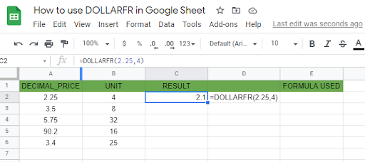
- The result in C2 now reads as 2 and 1/4. You can check that if you divide 1 by 4, you will get 0.25, which is the decimal part of our given constant.

- Notice that in this example, we provided the exact value, constant, as the arguments of our DOLLARFR. Alternatively, these constants can be variable or simply cell addresses of your data.
- Edit your function by changing the first and second argument into the cell addresses where your decimal_price and unit are located. In this case, cell A2 and cell B2.

- Copy the formula down to the remaining rows.

That’s pretty much it. You can now use DOLLARFR functions in Google Sheets together with the other numerous Google Sheets formulas to create even more powerful formulas that can make your life much easier.