How to Use IFERROR Function in Google Sheets

The IFERROR function in Google Sheets is used to effectively manage errors.

Instead of showing an error message, it assigns a value to show whenever an error is found.

The IFERROR function is a variation of the IF function that instructs the spreadsheet what to display when an error is encountered. It is also a more general version of the IFNA function, which is used when the #N/A error pops up.

Consider this example.

Say you were given the task of determining the average sales generated for each of the account managers by dividing the total sales by the quantity sold. The given data are as follows:

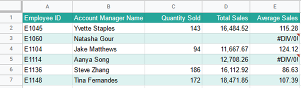
For the information that you do not have, you can choose to leave those blank and finish making the spreadsheet. After applying the formula for all the employees, you will notice a strange value pop up for those that have missing data. Upon selecting the cell containing this strange value, a note pops up that says, “Error Function DIVIDE parameter 2 cannot be zero.”

The reason for this error to show up is that the spreadsheet is trying to divide a value by zero. You still want to keep the formula present for when the missing data is inputted but would like to remove the strange value.

This is an instance where the IFERROR function is exactly what you are looking for. Instead of showing an error, it allows you to show a blank cell, a number, or even a custom message instead!

Encountering errors in Google Sheets is completely normal that even veteran users still receive these strange and cryptic-looking values from time to time! It seems intimidating and even discouraging for these strange combinations of symbols and letters to pop up when you’re unfamiliar with what they actually mean.

These prompts are not a random assortment of characters, but they actually provide the user a decent idea of what these errors are. Let me walk you through the different types of errors that you could encounter whenever you use Google Sheets.

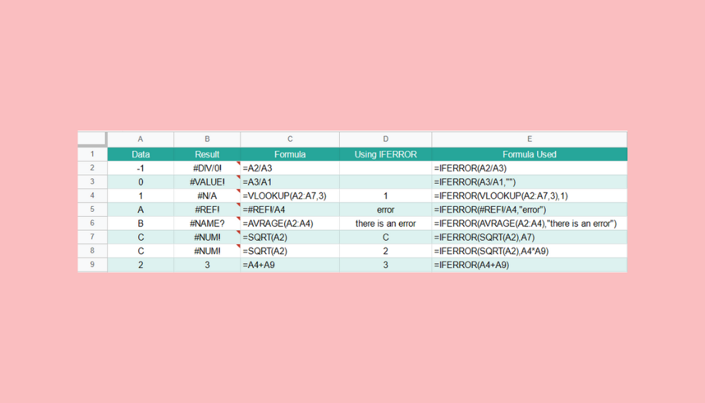
Different Types of Errors in Google Sheets

• #DIV/0 Error – this type of error shows up when a number is divided by zero
• #VALUE! Error – this error occurs when incorrect data types are used in a formula (i.e. having text involved in mathematical formulas)
• #N/A Error – called the “not available” error, this error occurs when a lookup formula is used, and the spreadsheet cannot find the value
• #REF! Error – called the reference error, this type of error shows up when the reference cell used in the formula is no longer valid or does not exist, usually a result of accidentally deleting rows or columns referenced in other cells
• #NAME? Error – this error shows up whenever Google Sheets does not recognize a function used in the formula, usually a result of misspelled functions (using IFEROR instead of IFERROR)
• #NUM! Error – this type of error occurs when the value calculated is either too large or is an invalid number (taking the square root of a negative number)

Still confused? Don’t worry! Examples for each type of error will be shown later. After a bit more exposure, these error messages will not seem as daunting as they are now.

No matter which kind of error you encounter, the IFERROR function is capable of replacing the error value with any value that you specify. Now, let’s finally learn how to use the IFERROR function to clean up those errors!

The Anatomy of the IFERROR Function

So the syntax (the way we write) the IFERROR function is as follows:

=IFERROR(value, [value_if_error])

Let’s dissect this thing and understand what each of these terms means:

• = the equal sign is just how we start any function in Google Sheets.
• IFERROR()  this is our IFERROR function. IFERROR will determine if the value returns any of the errors presented earlier. If it does, the function will show the value placed in the value_if_error argument and will keep the value argument if it does not.
• value is the first argument. This is the value that the function checks for errors. A cell reference or a formula may be used. If no error is detected, the function will return this value.
• value_if_error is the second argument. This is the value that the function returns if there is an error. A number, word, or text string may be used. The square brackets ‘[]’ indicate that this is an optional parameter. If left blank, the cell will display nothing (i.e., a blank cell).

A Real Example of using the IFERROR Function

Take a look at the example below to see how IFERROR functions are used in Google Sheets.

As you can see, the IFERROR function returns the original value in the first argument if no error is detected. For any kind of error, the value shown can be a blank, number, word, text string, cell reference, or even a formula.

You may make a copy of the spreadsheet using the link I have attached below: 🙂

How to Use IFERROR Function in Google Sheets

Let’s try to fix the example for calculating the average sales earlier so that the error message will not pop up while waiting for the missing data to be obtained.

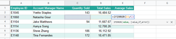
1. Simply click on any cell to make it the active cell. For this guide, I will be selecting E3, where I want to show my result.

2. Next, simply type the equal sign ‘=’ to begin the function and then followed by the name of the function, which is our ‘iferror’ (or ’IFERROR’, whichever works). You should find that as you are typing, an auto-suggest box appears with the names of the functions that contain the text that you have typed.

3. The one we want is the IFERROR function, so make sure to click on the IFERROR function. Alternatively, you may select the function by pressing the arrow down keys then pressing Enter or Tab to use the function (the currently selected function will be highlighted in grey and have a brief description below).

4. Upon selecting a function, a large text box appears that gives details about the function, and how to use the function. In some instances, a blue question mark will appear on the left side of the cell. If you want this text box to appear, simply click this question mark to show the large text box. Clicking on the arrow at the top right-hand corner will minimize the box while clicking on the x mark close the text box, and the blue question mark will appear.

5. The average sales shall be computed by dividing the total sales by the quantity sold. For now, let’s focus on calculating this value for row 3. Select cell D3, then press the forward slash ‘/’ key, and finally select C3. This is the formula for dividing cell D3 by C3. (Note: cell references are color-coded so you can easily distinguish which is being referenced in the formula)

6. Now, we can select what value will return if there is an error. I choose to leave a message saying “incomplete data” so that even a viewer can easily understand what is happening. To input this message, enter a comma ‘,’ after C3 to indicate that we are finished giving the value argument and would like to input the value_if_error argument. Then type “incomplete data”. For text, make sure that the message is enclosed in quotation marks and is highlighted in green as shown.

7. Finally, just hit the Enter key. You’ll find that the text “incomplete data” shows up in cell E3 instead of the #DIV/0 error.

8. To complete the table, simply copy the formula to the other rows.

NOTE:

Although the IFERROR function is a powerful tool in cleaning up errors that present themselves whenever working with Google Sheets, it does not give you an opportunity to determine the reasons why these errors occur. It simply hides the error, not address nor correct it.

I personally recommend only using it for the #DIV/0 error and some #N/A errors. For the other types, it would still be better to troubleshoot and fix the error to ensure that your spreadsheet will still work properly.

That’s pretty much it. You can now use IFERROR function in Google Sheets together with the other numerous Google Sheets formulas to create even more powerful formulas that can make your life much easier. 😀

Get emails from us about Google Sheets.

Our goal this year is to create lots of rich, bite-sized tutorials for Google Sheets users like you. If you liked this one, you'll love what we are working on! Readers receive ✨ early access ✨ to new content.

Subscribe