The UMINUS function in Google Sheets is used to change a number from positive to negative, and vice versa.
Table of Contents
This function is useful because it helps you to immediately reverse the sign of a given number. This is especially helpful when you are trying to create formulas with inputs given by a variety of people. For example, payments are usually just typed in by users as positive amounts, but for these numbers to work as intended for some finance formulas in Google Sheets, they need to be negative amounts. This will avoid broken formulas and mismatched information in your spreadsheets at the end of the day, which will make you run into some difficulties with your overall data in the long run.
Essentially, it’s the same thing as multiplying a value by -1, but in a much neater manner that allows analysts to check and track the validity of the formulas, you create in Google Sheets.
Let’s look at an example.
You have a spreadsheet that details the information on what several customers have been putting as donations for every month. They have been surveyed for their responses. Perhaps their entries are not formatted correctly, but some values are not available to be read and used in different calculations.
How should we go about this problem?
The UMINUS function takes in the input and reverses its given sign. Instead of scanning the entire spreadsheet and using arbitrary formulas that offer no explanation, this is a helpful tool that will allow for such a calculation to take place in a neat manner.
The Anatomy of UMINUS Function in Google Sheets
The syntax of the UMINUS function is as follows:
=UMINUS(value)
Let’s have a look at each part of the function to understand what is going on here:
=is the equals sign that starts off any function in Google Sheets.UMINUSis the name of our function.valueis the value to have its sign reversed, or alternatively, to be multiplied by negative 1 (-1).
A Real Example of Using UMINUS Function
Let’s look at the example below to see how to use the UMINUS function in Google Sheets.
Reversing Number Signs in Google Sheets
This is a simple problem. We want to reverse the sign of some numbers in a spreadsheet.
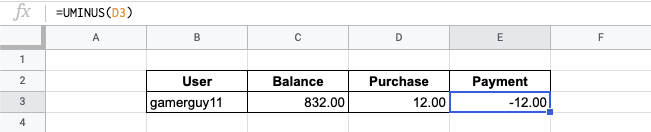
The function takes just one argument. So in the equation, it will look like:
=UMINUS(E3)
As a result, we get -12.
This simple problem can be practiced to perfection. Use the link below to get a copy of this problem set:
How to Use UMINUS Function in Google Sheets
In this section, we will show you a step-by-step process on how to use the UMINUS function in Google Sheets.
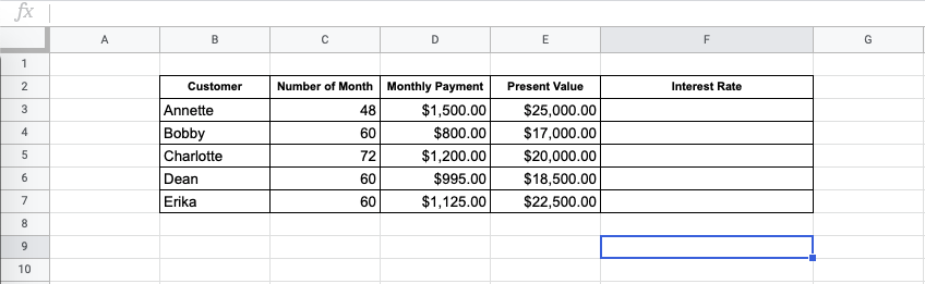
In this problem, we will fill the Interest Rate column using the RATE function, which requires a payment portion in the formula. To make the calculations easier, will use the UMINUS function to make logical shortcuts in the formulas that anyone using the spreadsheet can understand.
Using UMINUS within Finance Formulas In Google Sheets
- To begin, prepare your spreadsheet with the information you want to check.
- Start to fill in the
RATEfunction.

- Start to fill in the with the number of periods.

- For the payment attribute, we will use the
UMINUSfunction. Input the function name and then open bracket.

- Choose the cell that corresponds to the payment. This will be turned from a positive to a negative number, as the
RATEfunction requires.

- Next, finish off the
RATEfunction with the Present Value column.

- This formula is now done, and you should get the interest rate.

- Now, you can do it for the rest of the table, and you’re done!

The UMINUS function can help tidy up your spreadsheet. This should definitely help you avoid mistakes in your spreadsheets in the future, too.
And there you have it – you can now use the UMINUS function in Google Sheets together with the other numerous Google Sheets formulas to create even more effective formulas.