


Learning how to align imported data with manually entered data in Google Sheets is useful for effectively handling imported data.
Table of Contents
Working with imported data will always be a dynamic process as any changes made to the source data will affect your spreadsheet. This has the potential to cause problems, especially when working with both imported and manually entered data. Since most spreadsheet programs use formulas that are position-sensitive, any misalignments caused by updates to the source data could cause errors and ultimately ruin the spreadsheet.
In this article, we’ll learn how to align imported data with manually entered data in Google Sheets, whether the source data is from another Google Sheets file or another sheet from the same file.
Consider this example.
As a grocery store owner, it is important to keep track of your sales and perform an inventory of remaining stocks as frequently as possible. As such, you ask your employees to record daily sales and daily inventory in a spreadsheet file. Below is an example of a complete record.

You decide to create a separate spreadsheet that imports the data from this spreadsheet to calculate for profit generated for the sale of each product. In the new spreadsheet, you also decide to keep a record of previous days’ sales to determine whether to remove/replace some of the products you sell. A column for some comments to take note of for each product is also included.

This setup has been sufficient for the first few days of use; however, there will be days where the record would be rearranged (i.e. when a product is out of stock, the employee will not record it for that day, different order of products). Because of this, all of the calculations and notes you made on the separate spreadsheet are all mixed up. What can you do to fix this?
In this tutorial, we shall utilize unique IDs to group each row of data as part of a single record. These unique IDs will be used to relate the imported data with the manually inputted data. As such, we shall be making some changes to these existing spreadsheets as preparation for aligning imported data with manually entered data.
Creating Unique IDs
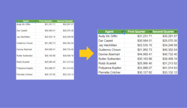
In the first spreadsheet, herein referred to as “SF1”, we shall add a column to assign an inventory ID for each food item. You may use any combination of characters as long as each ID is unique for each record.

For the second spreadsheet, which we will now refer to as “SF2”, let’s start working first in a separate sheet in the same file. This allows us to preserve the alignment of the imported and manually inputted data while we create some changes. Similar to SF1, create a column containing these unique IDs for SF2. It can be in any order, but it has to contain all the inventory IDs.

Since we have selected numbers as the IDs, we can sort them in ascending order. You may also add a few rows of additional IDs that may be used in the future.
To align these sets of data, we shall be depending on multiple functions, the VLOOKUP, IMPORTRANGE, IFERROR, and ARRAYFORMULA functions. We shall only discuss the first two functions in detail as they are the most essential to the task at hand while the latter two act more as shortcuts to make the task simpler. Follow the links to these functions for more detailed discussions.
Now, let’s first get to know more about the VLOOKUP function in Google Sheets!
The Anatomy of the VLOOKUP Function
So the syntax (the way we write) the VLOOKUP function is as follows:
=VLOOKUP(search_key, range, index, [is_sorted])
Let’s dissect this thing and understand what each of these terms means:
- = the equal sign is just how we start any function in Google Sheets.
VLOOKUP()this is ourVLOOKUPfunction. It searches down the first column of a range for a key and returns the value of a specified cell in the row found.search_keyis the value to search for.rangeis the array or range to consider for the search. The first column in the range is searched for the key specified insearch_key.indexis the column index of the value to be returned, where the first column inrangeis numbered 1.is_sortedindicates whether the column to be searched is sorted. It is an optional parameter, set to TRUE by default. Whenis_sortedis TRUE, the nearest match is returned. It is recommended, however, to set is_sorted to FALSE so that an exact match is returned.
The VLOOKUP function will be responsible for matching the unique IDs of each record to the correct row in SF2. This function will match the unique IDs (search_key) in SF2 to those in SF1 (range). It then returns values found in the same row. The index number specifies which data will be returned: 2 – Item, 3 – Category, 4 – Quantity in Stock, 5 – Sales.
Since we are working with imported data from another spreadsheet in this example, we would have to use the IMPORTRANGE function in the range parameter. As its name implies, this function allows us to import a range or array from a different file.
Now, let’s get to know more about the IMPORTRANGE function in Google Sheets!
The Anatomy of the IMPORTRANGE Function
So the syntax (the way we write) the IMPORTRANGE function is as follows:
=IMPORTRANGE(spreadhseet_url, range_string)
Let’s dissect this thing and understand what each of these terms means:
- = the equal sign is just how we start any function in Google Sheets.
IMPORTRANGE()this is ourIMPORTRANGEfunction. It imports a range of cells from a specified spreadsheet.spreadsheet_urlis the URL of the spreadsheet from which data will be imported. This value may either be enclosed in quotation marks or it may be a reference to a cell containing the URL.range_stringmust be a string value specifying the range to be imported. It must follow the format: ‘[sheet_name!]range’ (e.g. ‘Sheet1!A1:B3’ or ‘A1:B3’). If the sheet_name is not specified, theIMPORTRANGEfunction will import from the given range of the first sheet. The value forrange_stringmay either be enclosed in quotation marks or it may be a reference to a cell containing the URL.
Now that we have learned about the VLOOKUP and IMPORTRANGE functions, we are pretty much able to align imported data with manually entered data in Google Sheets. However, only using these two functions will require us to input a formula to every single cell in the spreadsheet where data is to be imported from. To make this task easier, we shall use the two additional functions mentioned earlier.
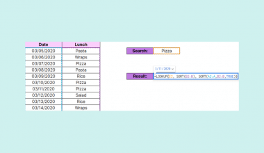
Using the ARRAYFORMULA function allows us to only input the formula for a single cell and it will return values for multiple cells. The IFERROR function allows us to remove errors that will arise from using a range in the formula that contains blanks. This results with the general formula:
=ARRAYFORMULA(IFERROR(VLOOKUP(Unique IDs,IMPORTRANGE(SF1 URL, Imported Data), index, FALSE)))
Now, we’re finally ready to align imported data with manually entered data in Google Sheets!
How to Align Imported Data with Manually Entered Data in Google Sheets
The steps laid out in this part of the tutorial refers to imported data from another spreadsheet file. Some notes will be discussed afterward on how to tweak the steps discussed below for data imported from the same file but in a separate sheet.
Let’s look at the scenario discussed earlier.
- Create unique IDs for each record in both of your spreadsheets. (Refer to the steps laid out in the “Creating Unique IDs” section of this tutorial). Edit sharing properties of SF1. Ensure that Anyone with the link is selected instead of Restricted.

- In SF2, simply click on any cell to make it the active cell. For this guide, I will be selecting B2 where I want to show my result. Next, type the formula: =ARRAYFORMULA(IFERROR(VLOOKUP(

- Next, select the first column as the
search_keyparameter or simply type A2:A. Afterward, type a comma ‘,’ to indicate that we would like to proceed to the next parameter. If done correctly, the first column except the header should be highlighted.

- For the
rangeparameter, we will use theIMPORTRANGEfunction. Type IMPORTRANGE or select the function as you are typing. Enclose the link of SF1 in quotation marks to input thespreadsheet_urlparameter. Next, specify the range containing the data to be imported. For this example, type “Inventory!A2:E” to select the first 5 columns. Finally, close therangeparameter with a close parenthesis and a comma. *Note: The “Inventory” in the formula refers to the sheet name in SF1 where you wish to retrieve data from.

- For the
indexparameter, specify the number of the columns you wish to import. In this example, we wish to extract all of the data in the range specified. Type {2,3,4,5} followed by a comma. The first column is not selected as it refers to the unique IDs. Type FALSE for theis_sortedparameter.

- Press Enter to complete the formula. Return the data from earlier to their corresponding alignments.

Lastly, here are some things that you need to take note of:
- It is important that the IDs used are unique for each record and are used properly and consistently to avoid errors later.
- In SF2, columns B to F consist of imported data. You should avoid putting manually entered data for these columns as it will result in an error.
- Even if some IDs in SF1 are deleted or not present, the same ID will still be present in SF2 but columns containing imported data will be blank.
- For imported data from the same file, simply replace the
IMPORTRANGEfunction with the range in the [sheet_name!]range format. The general formula then will be:
=ARRAYFORMULA(IFERROR(VLOOKUP(Unique IDs,[sheet_name]!range, index, FALSE)))
We’re done! It’s easy to align imported data with manually entered data, right?
If you want to practice some more, make a copy of our spreadsheets and give it a try:
Or browse our other numerous Google Sheets formulas to create even more powerful formulas that can make your life much easier.


2 comments
Hi! I am trying to do something similar for my current job. When someone calls out of a shift, their Google Form responses (dynamic data) are imported to another spreadsheet where other employees can add their name to claim the shift (static data). I am trying to set it up where only future shifts will be shown in the second spreadsheet. This is easy, but every day when the list is updated automatically, the static names don’t move with the dynamic shifts. I have added IDs to the responses to align the data. However, as you mentioned, “Even if some IDs in SF1 are deleted or not present, the same ID will still be present in SF2 but columns containing imported data will be blank.” How can I solve this?
I have tried using a filter function to remove the blank rows, but I can’t seem to make it work. Because I had to create “IDs” for all future form responses (1-9999), those rows exist in the second spreadsheet but are blank once the shift has passed. How can I remove the blank rows from the vlookup output? Thank you so much in advance!
As the IDs are Static in destination Sheet we are using VLOOKUP. But if the IDs are Dynamic then Can we link Static Data or Manually added columns.