The ERROR.TYPE function in Google Sheets is useful if you want to identify the type of error values in a specific cell by returning the error numbers in another cell.
Meaning, the ERROR.TYPE function will return the number of days between two dates as a year fraction in decimal format.
Table of Contents
The rules for using the ERROR.TYPE function in Google Sheets are as follows:
- The ERROR.TYPE function can use an indirect argument, which is a cell reference to a formula.
- The ERROR.TYPE function can also use a direct argument, which is a formula.
- The ERROR.TYPE function will either return a number from 1-8 or the $N/A error.
- The numbers 1-8 correspond to error types. If no error exists, ERROR.TYPE returns #N/A.

Let’s take an example.
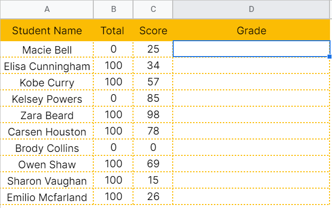
Chad is a technical instructor who teaches Google Sheets function in college. He asked help from his brother to key in some student information to his class records. However, he checked his work and encountered some minor issues in his calculations.
See his students’ record below:

Chad wants to create a formula that would remind his brother on how to fix the #DIV/0 in column D.
Using the combination of the IF, IFNA, and ERROR.TYPE functions, he was able to identify the instances of #DIV/0 error and return a text to remind his brother on how to deal with them.
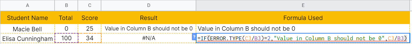
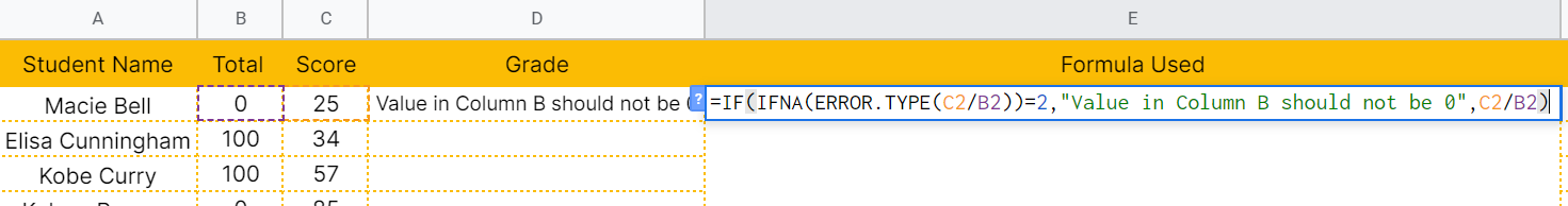
See his updated table below:

This way, his brother can easily fix the error before the file gets to him.
Pretty smart, right?
Watch out for a more advanced tutorial and examples on how you can use the ERROR.TYPE function in the coming weeks. Be sure to subscribe to be notified.
Awesome! Let’s begin getting to know more about our ERROR.TYPE function in Google Sheets.
The Anatomy of the ERROR.TYPE Function
So the syntax (the way we write) of the ERROR.TYPE function is as follows:
=ERROR.TYPE (error_val)
Let’s dissect this thing and understand what each of these terms means:
- = the equal sign is just how we start any function in Google Sheets. It is how Google Sheets understand that we are asking it to either do computation or use a function.
- ERROR.TYPE() this is our ERROR.TYPE function. It returns the error number or #N/A if no error.
- error_val is the only argument and the error for which to get an error code.
A Real Example of Using ERROR.TYPE Function
Let’s take a look at Chad’s table below to see how the ERROR.TYPE function is used in Google Sheets.

The ERROR.TYPE function identifies the type of error, if any, that a certain calculation or formula would return. If the calculation doesn’t return any error, the ERROR.TYPE function would return the #N/A error.
Like what Chad did on the file, one way to utilize ERROR.TYPE is to test for specific errors and display a relevant prompt or message, instead of error values, when certain error conditions exist.
In the examples above, Chad used the combination of the IF, IFNA, and ERROR.TYPE functions to satisfy what he needs for catching errors. The ERROR.TYPE would return either the prompt message he assigned or the calculation he needs.
The ERROR.TYPE function needs only one argument to perform its job. That’s the error_val or the value to be tested.
In the first example above, the argument used is a calculation to find the quotient of two cell references, which are C2 and B2.

We know that the division would either result in an error or the quotient of the two numbers.
What could result in an error?
Remember that any number divided by a 0 is undefined and for Google Sheets, it’s a #DIV/0! error.

Now, it will return the corresponding number, instead of the #DIV/0! Error, if we pass this calculation to the ERROR.TYPE function.

The integer 2 corresponds to #DIV/0! in the ERROR.TYPE function.
This number now can be used for the IF function, which is used if you want to test whether a certain condition is true or false.
If you want to know more about the IF function, its definition, and examples, feel free to visit this article.
Going back, as we mentioned above, one way to utilize ERROR.TYPE is to test for specific errors and display a relevant prompt or message, instead of error values.
In this case, we will test each calculation of columns B and C using the ERROR.TYPE function. If it returns 2, then it means the calculation yields the #DIV/0! error. Once it does, we will ask our IF function to return the message “Value in Column B should not be 0.”

But, what would happen if the calculation doesn’t yield the #DIV/0 error?
That’s something we can provide the IF function as its third argument.
=IF(logical_expression, value_if_true, value_if_false)
In this case, we can simply ask the IF function to perform the calculation nonetheless.

However, it looks like the IF function doesn’t allow it if the logical_expression returns the #N/A! error as the IF function itself will return the #N/A! error. Please note that if our ERROR.TYPE found no error in its argument, it would return the #N/A! error.
For the IF function can proceed, we will create a workaround.
This is where the IFNA function will come in handy. For more information about the IFNA function, its definition, and examples, feel free to visit this article.

Using the IFNA function, we will first test whether our ERROR.TYPE function will return an #N/A or not. If it does, the IFNA function will return a null value, that is “”, which will be passed to our IF function for consumption.
The logical_expression in the IF function will either return the value 2 or a null value. If it’s 2, then it will provide us the message we assigned, otherwise, it would just proceed to calculate the quotient of columns C and B.
You may make a copy of the spreadsheet using the link I have attached below.
How to Use ERROR.TYPE Function in Google Sheets
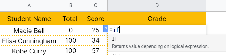
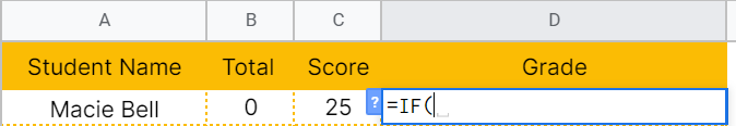
- Click on any cell to make it the active cell. For this guide, I will be selecting D2, where I want to show the result.
- Next, type the equal sign ‘=‘ to begin the function and then follow it with the name of the function. We will be using nested functions in our example below. So first, type in ‘if‘ (or ‘IF‘, not case sensitive like our other functions).
- Type open parenthesis ‘(‘ or simply hit Tab key to let you use that function.
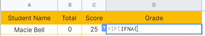
- Now the exciting part! Let’s give our IF function its first argument, which is the IFNA function. Type in ‘ifna’ or ‘IFNA’ then hit the Tab key.
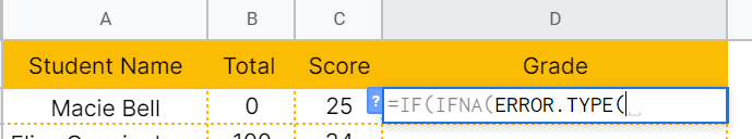
- Type in the only argument of IFNA function in this case, which is our ERROR.TYPE function. Type in ‘error.type’ or ‘ERROR.TYPE’ then hit the Tab key again.
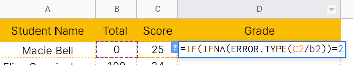
- Next, type in the only argument for our ERROR.TYPE function, which is the error_val. Type in ‘C2/B2’ and a closing parenthesis ‘)’.

- End the IFNA function by typing in another closing parenthesis ‘)’.

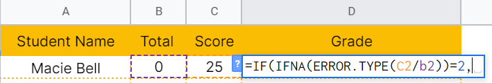
- Now, continue the first argument of the IF function by typing in equal sign ‘=’ and the value 2.
- To let the Google sheet know that we’re done typing our first argument for the IF function, we should now type in the delimiter or the character that separates each argument on a function. In this case, type comma ‘,’.
- The second argument of the IF function is what we want it to do if the first argument returns TRUE. In this case, we want it to return a specific message. Type in ‘Value in Column B should not be 0’ and follow it with a comma (,). Since the second argument is a string, we will need to enclose it with quotation marks (“”).

- The third argument of the IF function is what we want it to do if the first argument returns FALSE. We want it to just proceed with the calculation in this example. Type in ‘C2/B2’.

- Finally, hit your Enter or Tab key. Cell D2 will now show you the return value of our nested functions.
- Copy the formula down to the remaining rows.

That’s pretty much it. You can now use the ERROR.TYPE function in Google Sheets together with the other numerous Google Sheets formulas to create even more powerful formulas that can make your life much easier.