How to Use NPV Function in Google Sheets

The NPV function in Google Sheets is a useful tool to help determine the net present value of an investment, based on a series of cash flows and a discount rate. If you are interested in a certain investment, you should study it and understand how you can benefit from it in the future against certain scenarios. The NPV function can you help you do that.

The NPV function is used to find the net present value of an investment. The net present value is a term in finance that refers to the difference between the current value of cash inflows and outflows. This tool is usually used when encountering investment due diligence and capital budgeting, in order to make good decisions on the value of a project versus other options.

Let’s look at an example.

Your company is deciding which project to pursue, investment-wise. You have the information about each project’s inflows and outflows, as well as the discount rate.

How should you approach this problem?

The NPV function needs you to set up the cash flows, as well as know your rates in order to study each project and make a sound financial decision. From there, you can compare the two results and decide which project is best for the company.

The Anatomy of the NPV Function in Google Sheets

The syntax of the NPV function is as follows::

=NPV(discount, cashflow1, [cashflow2,...])

Let’s have a look at each part of the function to understand what is going on here:

• = is the equals sign that starts off any function in Google Sheets.
• NPV is the name of our function.
• discount is the discount rate of investment over one period.
• cashflow1 is the first future cash flow.

Note that NPV is similar to PV, except that variable cash flows are allowed in NPV. If your problem encounters irregular cash flows, choose to use XNPVinstead.

You should also note that the perspective you are solving the problem from also matters.

If you are the owner of the investment, the cashflow1and any subsequent cashflows will represent income, so they should be positive.

If you are the perspective of someone making a loan repayment, the cashflow1and any subsequent cashflows will represent payments, so they should be negative.

When the net present value is zero, the internal rate of return under the same conditions is the discount rate.

A Real Example of Using the NPV Function

Let’s look at the example below to see how to use NPV function in Google Sheets.

Calculating the Net Present Value in Google Sheets

This is a simple problem. We want to find the net present for a certain project. Here in the example, the cash flow is laid out, as well as the discount rate.

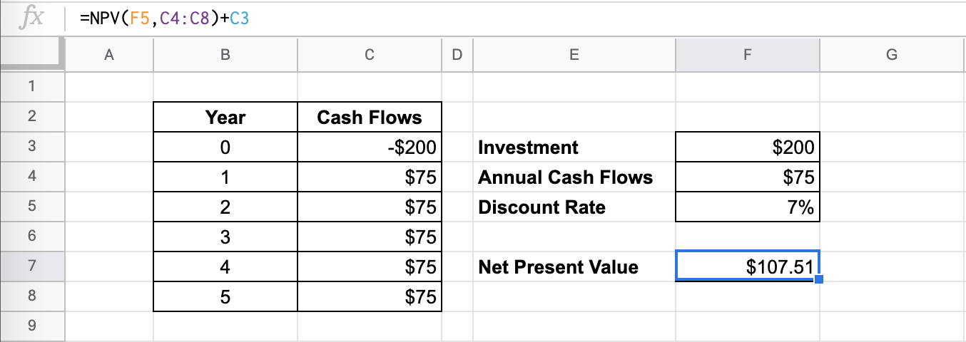
In this example, the function NPV will take 2 arguments. So in the equation, it will look like:

=NPV(F5,C4:C8)

As a result, we get $307.51.

However, since we are looking for the Net Present Value, we need to remove the Initial Investment of $200. So as a result, the Net Present Value will be $107.51.

This simple problem can be practiced to perfection. Use the link below to get a copy of this problem set:

How to Use the NPV Function in Google Sheets

In this section, we will show you a step-by-step process on how to use the NPV function in Google Sheets.

In this problem, we will be comparing two different projects. The information that you have is laid out over two different cases. They are all projects that are not easy to compare at first glance because they have different costs and different cash flows to offer the company.

It’s up to you, as the project manager, to decide which project will benefit the company the most. You have decided to use the NPV to compare these projects and evaluate them after you have calculated for their NPVs.

Calculating and Comparing NPV in Google Sheets

1. To begin, click on a cell to make active, which you would like to display the MIRR. For the guide. The NPV will be in Cell F7. Start to type the name of our function, which is NPV.
   
2. The auto-suggest box will create a drop-down menu. Select the NPV function by clicking it. It is the first to pop up on the list, but take care to choose the correct function.
   
   
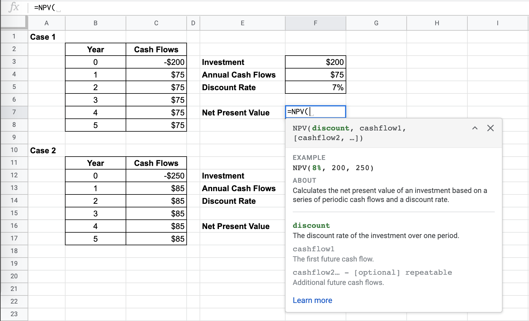
3. After the opening bracket ‘(‘, you will add the discount rate attribute. You can either type down the discount rate, or use a cell reference. In this example, we used the cell reference by clicking on F5.
   
4. Now you will add the range attribute. You can either type down each cash flow, or use a cell reference. In this example, we used the cell reference by clicking and dragging on C4:C8.
   
5. You will notice that there will be a preview of the result when you complete the inputs. But you’re not done yet!
6. Since we did not consider the initial investment or payment when purchasing the project, what we have is just the Present Value, or PV of the project. We need to subtract the initial investment from the calculation. In this example, we used the cell reference by clicking on XX.
   
7. Close off with another bracket and hit enter.
   
8. Go through the steps for the next example.
   
9. You should be able to compare the two projects and the project with a greater Net Present Value should be your choice.
   

And there you have it – you can now use the NPV function in Google Sheets together with the other numerous Google Sheets formulas to create even more effective formulas.

Get emails from us about Google Sheets.

Our goal this year is to create lots of rich, bite-sized tutorials for Google Sheets users like you. If you liked this one, you'll love what we are working on! Readers receive ✨ early access ✨ to new content. There will be no spam and you can unsubscribe at any time.

Subscribe