This guide will discuss how to use the COUNTUNIQUEIFS function in Google Sheets.
When we need to return the unique count of a range depending on multiple criteria, we can easily do this using the COUNTUNIQUEIFS function in Google Sheets.
Table of Contents
The rules for using the COUNTUNIQUEIFS function in Google Sheets are the following:
- If none of the criteria are satisfied, the
COUNTUNIQUEIFSfunction will return 0. - The count_unique_range and all the criteria_range arguments must contain the same number of rows and columns. Otherwise, the function will return a #VALUE! error.
Google Sheets has several built-in functions that we can utilize to count unique values in a large data set easily. For example, the UNIQUE function, the COUNTUNIQUE function, and the COUNTIF function.
The COUNTUNIQUEIFS function is a newly released function that conditionally counts the unique values in a range if provided conditions match the additional ranges.
Previously, we would have to combine two functions to conditionally count unique values. For instance, we would combine the COUNTUNIQUE function and the Filter tool.
The COUNTUNIQUEIFS is a simplified function that allows us to conditionally count unique values efficiently.
In this guide, we will provide a step-by-step tutorial on how to use the COUNTUNIQUEIFS function in Google Sheets. Additionally, we will explore the syntax and a real example of using the function.
Great! Let’s dive right in.
The Anatomy of the COUNTUNIQUEIFS Function
The syntax or the way we write the COUNTUNIQUEIFS function is as follows:
=COUNTUNIQUEIFS(count_unique_range,criteria_range1,criterion1,[criteria_range2,criterion2, …])
- = the equal sign is how we activate any function in Google Sheets.
- COUNTUNIQUEIFS() is our
COUNTUNIQUEIFSfunction. This function is used to count the unique values of a given range depending on multiple criteria. - count_unique_range is a required argument. This refers to the range from which the unique values will be counted.
- criteria_range1 is another required argument. This refers to the range to check against the criterion1 argument.
- criterion1 is also a required argument. This refers to the pattern or test to apply to criteria_range1.
- criteria_range2 is an optional argument. This is the additional ranges we want to check.
- criterion2 is also an optional argument. This is the additional pattern or test we want to apply.
Note: The COUNTUNIQUEIFS function is only available in Google Sheets. The function is not available in Excel.
Understanding the COUNTUNIQUEIFS Function Arguments
The COUNTUNIQUEIFS function is a method of filtering multiple columns for unique values. We can compare columns with greater than or less than. Hence, we can do anything else with the IFS function.
Additionally, this is a useful tool when we need to highlight or remove duplicate items in a spreadsheet. Moreover, it is also helpful to track what we have and have yet to accomplish.
The count_unique_range argument is the range we want to count the unique data. Then, the criteria_range1 argument is the range where we apply the given conditions or criteria. Moreover, we can supply additional ranges and criteria.
However, we only need one criterion for the function to work properly.
Firstly, the COUNTUNIQUEIFS function will filter the given count_unique_range by applying the criterion1 argument. Then, the function will count the unique entries in the coun_unique_range that match the given criteria.
The criteria we can use can be equal to a specific value, greater than or greater than or equal to, and less than or less than or equal to.
A Real Example of Using COUNTUNIQUEIFS Function in Google Sheets
Let’s say three people took a test, and their scores have been recorded. Each person has three scores since they took the test three times. Our initial data set would look like this:

In the spreadsheet above, we can see that the data was not organized into separate columns per person. In this example, we want to find the count of unique scores of each person.
We will apply the formula below to complete this task:
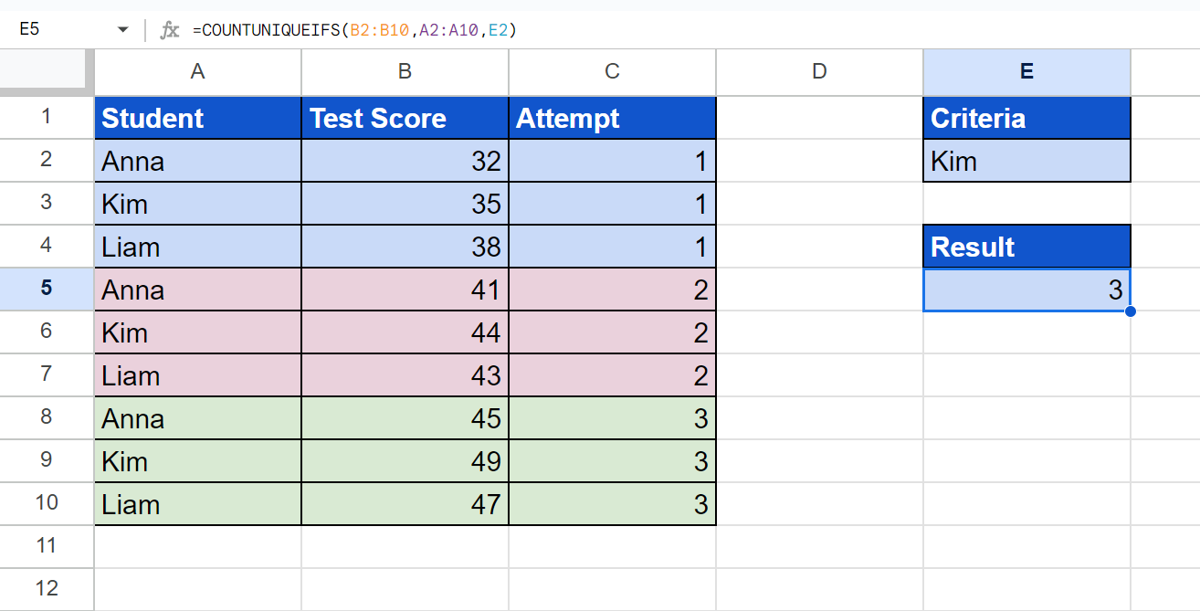
=COUNTUNIQUEIFS(B2:B10,A2:A10,E2)

The first part of the formula is our count_unique_range argument which is the range B2:B10. Next, we simply selected the range A2:A10 as our criterion1 argument. Lastly, we selected cell E2 which contains the criterion1 argument.
Our final data set would look like this:

You can make your own copy of the spreadsheet above using the link below.
Amazing! Now we can dive into the steps of using the COUNTUNIQUEIFS function in Google Sheets.
How to Use COUNTUNIQUEIFS Function in Google Sheets
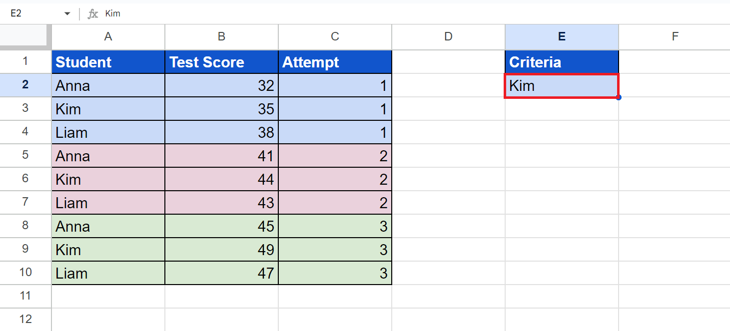
1. First, we will select an empty cell and input our criteria. In this case, the criteria are the name of the person who took the test, such as Anna or Kim.
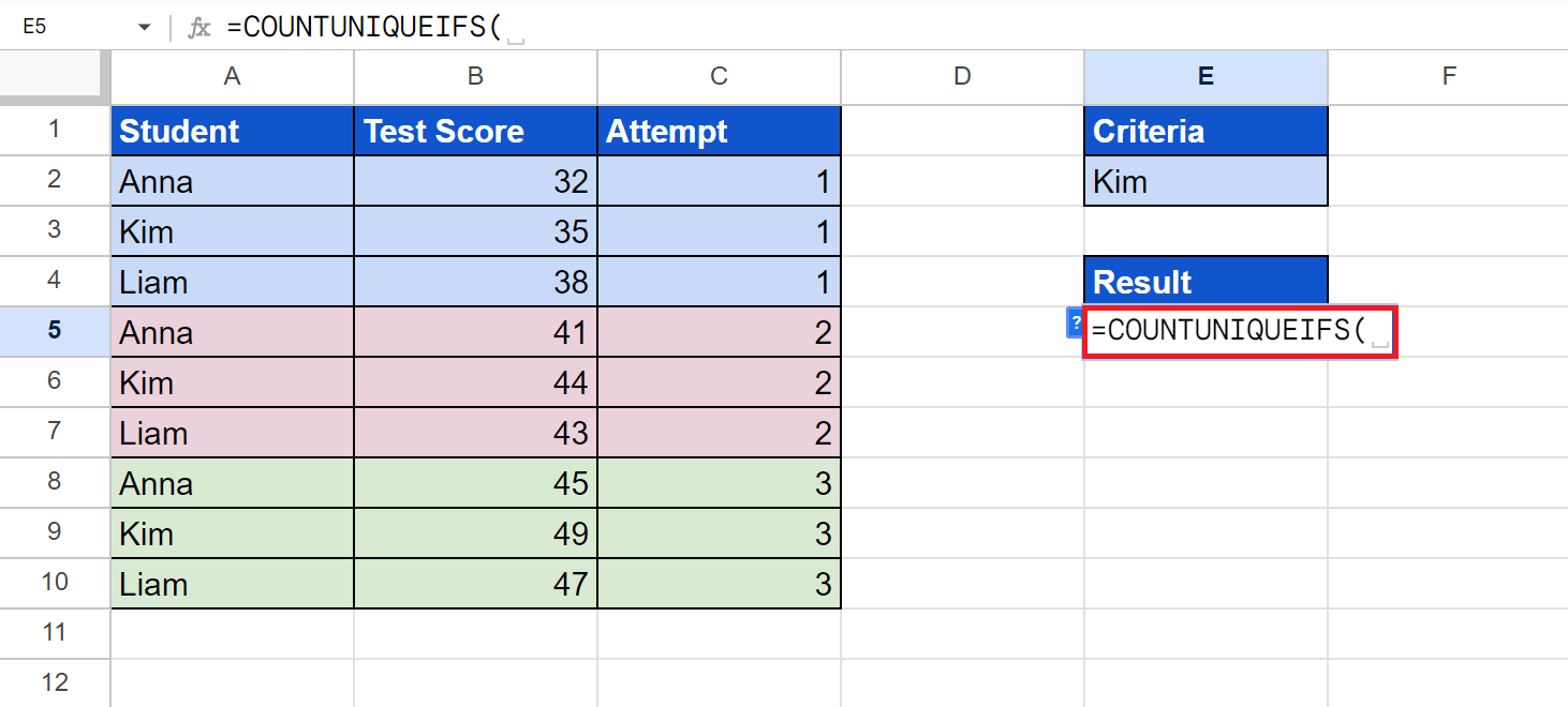
2. Then, we will select another empty cell to display the result. To begin, we will type in an equal sign and the function name. Our formula would be “=COUNTUNIQUEIFS(”.
3. Next, we will select the range where we want to count the unique values. Our formula would be “=COUNTUNIQUEIFS(B2:B10”.

4. Afterward, we will highlight the range where we apply the criteria. Thus, our formula would be “=COUNTUNIQUEIFS(B2:B10,A2:A10”.

5. Lastly, we will select the cell containing the criteria. Our final formula would be “=COUNTUNIQUEIFS(B2:B10,A2:A10,E2)”.

However, we can also directly type the name enclosed in double quotes. For instance, the final formula would be “=COUNTUNIQUEIFS(B2:B10,A2:A10,”Kim”)”.
6. We will press the Enter key to return the result.
And tada! We have successfully used the COUNTUNIQUEIFS function in Google Sheets.
You can apply this guide whenever you need to calculate the variance of a sample. You can now use the COUNTUNIQUEIFS function and the various other Google Sheets formulas available to create great worksheets that work for you.
FAQs
1. Is there an alternative method to conditionally count unique values in Google Sheets?
The COUNTUNIQUEIFS function is a relatively new function that conditionally counts unique values. Previously, we would have to combine functions to count unique values conditionally.
For example, we can utilize the COUNTUNIQUE function + Filter tool together. Another is we can also use the UNIQUE function, the COUNTUNIQUE function, and the COUNTIF function.
2. What are the common COUNTUNIQUEIFS errors?
If the result is 0, none of the given range values matches the criterion set.
If the function returns a #VALUE! error, the count_unique_range and criteria_range1 may have different sizes. Ensure all the given ranges have the same dimensions.
That’s pretty much it! Make sure to subscribe to our newsletter to be the first to know about the latest guides and tutorials from us.