How to Use IF within the FILTER Function in Google Sheets

Knowing how to use IF within the FILTER function in Google Sheets is useful if you would want to skip filtering a table if the condition is blank.

Normally, when you write the FILTER formula with the blank criterion, it would filter rows containing blank cells in the corresponding column.

Let’s take an example!

Say you have a list of products, with their categories and prices. However, not all of the products have their price listed 🍎🍍🥔

Let’s now say that our criterion is in cell D1 and it is 5. If you write the FILTER formula like this =FILTER(A2:C11,C2:C11<=D1), where C is the column with the prices, it would filter rows with the price lower than or equal to our criterion (in cell D1), which is 5. If we remove the criterion from the cell D1, the FILTER formula would filter rows with blank cells in column C. But let’s say we want the entire table as the filtered output if the criterion is blank.

So how do we do that?

Easy. This is where we will use the IF statement within the FILTER Function in Google Sheets.

Let’s first take a look at the anatomy of the single condition IF and FILTER combination to help you better understand how to use IF within the FILTER function in Google Sheets.

The Anatomy of the Single Condition IF and FILTER Combination in Google Sheets

The syntax (the way we write) the FILTER function is as follows:

Let’s break this down and explain each of these terms.

= the equals sign is the sign we put at the beginning of any function in Google Sheets.
FILTER() is our function. We will have to add the following variables into it for it to work.
range is the data to be sorted.
condition1 is a column or row containing TRUE or FALSE values corresponding to a selected column or row of the range. The function must have at least one condition.
condition2, … are additional conditions you can add if you need to check more than one condition.

In this guide, our condition is the IF function. The syntax (the way we write) the IF function is as follows:

Let’s break this one down, too!

= as said before, the equals sign is used at the beginning of any function in Google Sheets.
IF() this is our IF function. To make it work, we will have to add our logical_expression, value_if_true, and value_if_false inside the round brackets.
logical_expression is the condition that we want to test to see whether it is true or false.
value_if_true is the operation (the work to be done) that we want to carry out if the logical_expression is tested to be true
value_if_false is the operation (the work to be done) that we want to carry out if the logical_expression is tested to be false.

When we have a single condition IF and FILTER combination, our formula will look like this:

A Real Example of the Single Condition IF and FILTER Combination in Google Sheets

Take a look at the example below to see how the single condition IF and FILTER combination is used in Google Sheets.

We have a list of products (in column A), with their categories (in column B) and prices (in column C). As we can see, some products do not have their price listed.

Let’s say that we want to filter the products with prices lower than or equal to 5. Our criterion (5) is in cell D1, so our formula will look like this =FILTER(A2:C11,C2:C11<=D1). We will paste this formula in cell E2 and it will filter the rows with the price (in column C) lower than or equal to 5.

But what will happen if we remove the criterion from the cell D1?

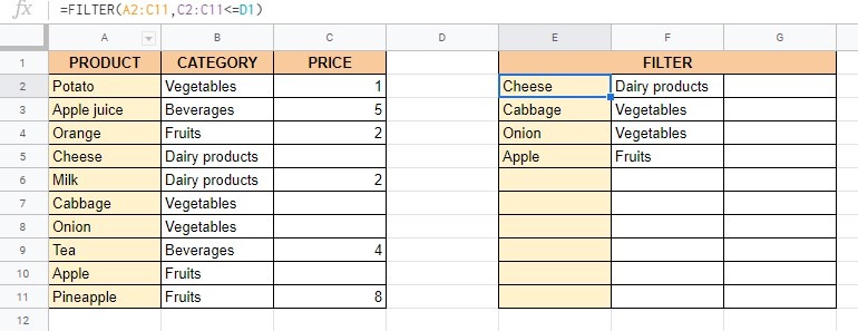
As you can see, the formula would filter the rows with blank cells in column C.

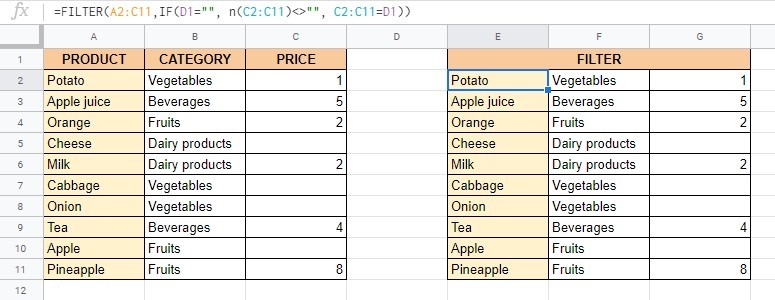
But what if now we want the entire table as the filtered output if the criterion is blank? This is where we will use the single condition IF and FILTER combination.

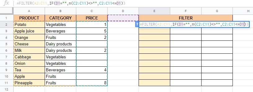
We will enter the following formula =FILTER(A2:C11,IF(D1=””, n(C2:C11)<>””, C2:C11<=D1)) in cell E2 and it would filter the entire table instead of just rows with blank cells in column C.

How to Use the Single Condition IF and FILTER Combination in Google Sheets

Let’s begin writing your own single condition IF and FILTER combination in Google Sheets, step-by-step.

1. First, make sure that the area where you would want to put your filtered data is empty. If so, click on a cell where you would enter the formula to make it active. This time, we will use the cell E2.

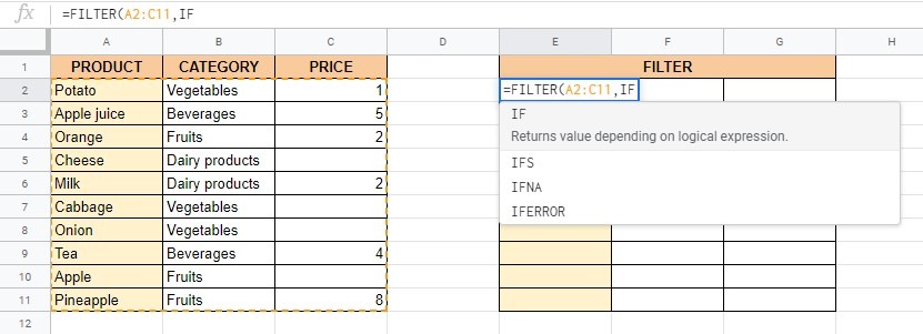
2. Start the function with the equals sign ‘=’ and type the name of the function, which is FILTER. As you start typing, you will get auto-suggestions with functions that start with the same letters. Choose the FILTER function from the suggestions or continue typing.

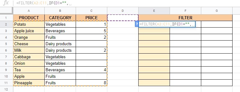
3. After the opening round bracket ‘(‘ we will enter our range, which is A2:C11. Put a comma ‘,’ after it.

4. Now we should enter our other function, which is IF.

5. Enter the opening round bracket ‘(‘ and our logical_expression, which is D1=””. Put a comma ‘,’ after it.

6. Now we should enter our value_if_true which is n(C2:C11)<>”” meaning that if cell D1 is empty, the formula should filter all the rows in range C2:C11 which are lower or higher than cell D1. Put another comma ‘,’.

7. And finally, we should enter the value_if_false which is C2:C11<=D1 meaning that if cell D1 is not empty, the formula should filter all the rows in range C2:C11 which are lower or equal to cell D1. Enter two closing round brackets ‘))’ to close the function and hit the Enter key on your keyboard.

8. If you did everything right, the formula would filter the entire table (A2:C11) since the cell D1 is empty.

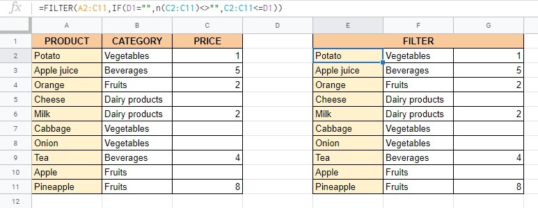
That’s it! Now you know how to use the single condition IF and FILTER combination in Google Sheets!

You can make a copy of the spreadsheet using the link below and practice some more before continuing to the multiple conditions IF and FILTER combination in Google Sheets:

The Anatomy of the Multiple Conditions IF and FILTER Combination in Google Sheets

The syntax (the way we write) the formula for multiple conditions IF and FILTER combination is similar to the one with the single condition, and is as follows:

As you can see, the only difference is that now we have two conditions.

A Real Example of the Multiple Conditions IF and FILTER Combination in Google Sheets

Let’s go back to our products! 🍎🍍🥔

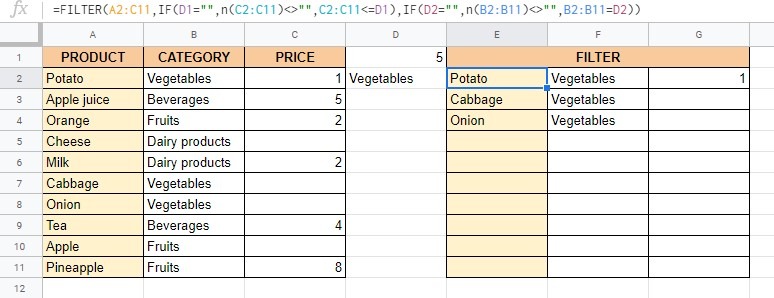
Once again, we will filter our products by the price but this time we will also filter them by category. As you can see, we will look for all the ‘Vegetables’ (cell D2) that are priced lower than or equal to ‘5’ (cell D1).

But what if the cells D1 and D2 were blank? The above formula would filter the entire table. Let’s take a look at how to do this!

How to Use the Multiple Conditions IF and FILTER Combination in Google Sheets

The first few steps are the same as the ones for the single condition IF and FILTER combination in Google Sheets. Just instead of two closing round brackets ‘)’ this time we will enter just one, and add another condition. The second condition is IF(D1=“”,n(C2:C11)<>“”,C2:C11<=D1) so our formula will look like this =FILTER(A2:C11,IF(D1=“”,n(C2:C11)<>“”,C2:C11<=D1),IF(D2=“”,n(B2:B11)<>“”,B2:B11=D2)).

If you did everything right, the formula would filter the entire table (A2:C11) since both cells, D1 and D2 are empty.

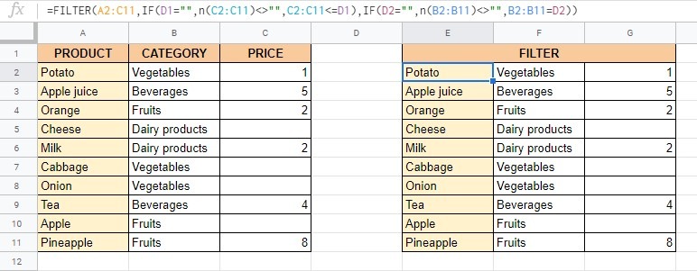
That’s it! Now you know how to use the multiple conditions IF and FILTER combination in Google Sheets, as well!

Take a look at the other Google Sheets formulas you can use to create even more effective formulas! 🙂

Get emails from us about Google Sheets.

Our goal this year is to create lots of rich, bite-sized tutorials for Google Sheets users like you. If you liked this one, you'll love what we are working on! Readers receive ✨ early access ✨ to new content.

Subscribe