How to Find the Highest N Values in Each Group in Google Sheets

This guide to find the highest N Values in each group in Google Sheets is useful if you want to find the top-ranking items in the first n places within an array.

This is especially helpful if you have a dynamic sheet where the values constantly change, and it’s important to keep up with the top-ranking entries for your monitoring purposes.

Let’s look at an example.

You are a class monitor and your job is to collect the grades of a class for every quiz, and post an update of students and their scored quizzes they have collected thus far. Your task is to keep track of the top two scored quizzes of each student that counts towards their final score, which changes often due to additional requirements.

In this problem, we consider each student as a group and the top 2 highest quiz scores as the highest 2 values.

You want to have a formula that will announce the top 2 quizzes of each student immediately after inputting the new scores that can potentially change rankings. It will also help students keep track of their grades and aim for a score that will help their final grade.

How might we go about that?

It’s as simple as finding the highest 2 values for each group within the array.

For this problem, you might be tempted to use RANK, MAX, or a combination. However, this solution also offers a straightforward method.

This solution will use a combination of QUERY, SORT, ROW, and MATCHfunctions to find our highest N values. This formula will run a Google API that simplifies data analysis, sort through, and find the correct values and find the corresponding group that matches said values.

Not to worry if the formula doesn’t make sense yet. By the end of this article, you will understand what each part of the formula does, so just keep your mind open and patient as you learn each portion step-by-step.

The Anatomy of the QUERY Function

The syntax (the way we write) the QUERY function is as follows:

=QUERY(data,query,[headers])

Let’s break the formula down to understand what is being required in each portion:

• = the equal sign is how we start all the functions in Google Sheets
• QUERYis our function. We need to provide the data, query, and optional headers.
• data is the range of cells to perform the query on. Note that each column of data should be of the numeric, string, or Boolean type. If a column mixes data types, it will execute the query considering the majority data type of the column, where other data types are considered as null.
• queryis the query to perform as written in the Google Visualization API Query Language. It should be a value enclosed in quotation marks, or a cell reference containing the appropriate text.
• headers are [OPTIONAL], and it indicates the number of header row on top of the data. If you don’t fill it up, it is set as a guess according to the data contents.

A Real Example of Using QUERY Function

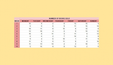
Have a look at the example to see how you can use the QUERY function to find the data that you need in a complex spreadsheet. Let’s see this class list and see which students have submitted their final projects.

The above image shows how to use the QUERY function to find the desired data among the different details within the array. The function is as follows:

=QUERY(A2:E21,"Select A, C, D, E WHERE E='No'")

After you input this formula, Google Sheets will run (don’t be surprised, it may take a while to load the results you are looking for) and instantly populate the cells with the subset of the array that you needed. Note that the query is an actual instruction, wrapped in quotation marks. It has some getting used to, but the powerful QUERY function can be very intuitive with a lot of practice!

Here is what this example does:

• We wrote our QUERY function with the variables separated by commas.
• We prepared a cell for the formula to output the subset we want to find, extracted from the larger set. In the example, we prepared the headers we want, and input the function in cell G2. Note that this is the only cell you need to manipulate.
• The first variable is the data range. Therefore, we selected the range of the entire set, including the headers. Here we input A:E.
• The second variable is the query. It is part of the Google API, and you can read more about the possible English-language queries to insert in this portion of the formula. For this example, we simply want the ID, Last Name, Class slot, and whether the student submitted their final project. We write, in double quotation marks, “Select A, C, D, E WHERE E=’No’”. Note what data each column letter refers to, and how in the final column, the requirement as a string was inputted with single quotation marks.
• You can also add more items to the list. If you adjust the range, then your list will automatically populate.

With some practice, you will be familiar with how the QUERY function works.

Make a copy of the spreadsheet from the link attached below and try it for yourself:

How to Find the N Highest Values in a Group in Google Sheets

Here is a step-by-step process to find the n highest values in a group in Google Sheets using the QUERY function combined with SORT, ROW, and MATCH.

1. To start, select the cell where you want to show the result of your query. Make sure there is enough space to the right of the cell to populate. In the example, We chose cell G3.

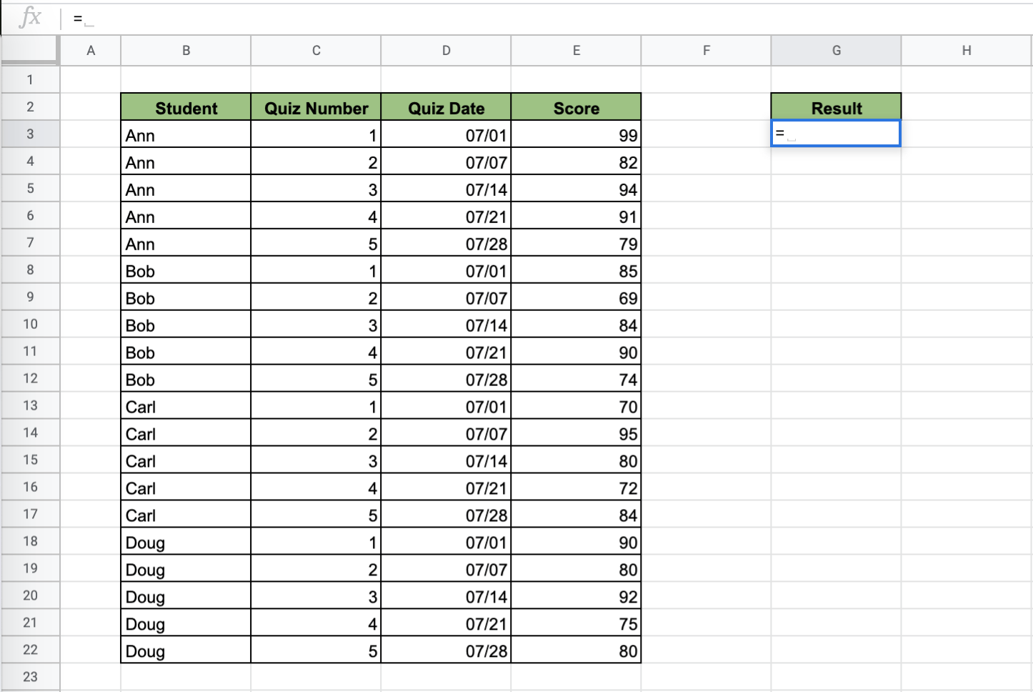
2. Since we are working on a query that deals with more than 1 desired result (in this case, we want the n = 2 highest scores, we must use the ARRAYFORMULA function. Enter the equal sign and look for ARRAYFORMULA.

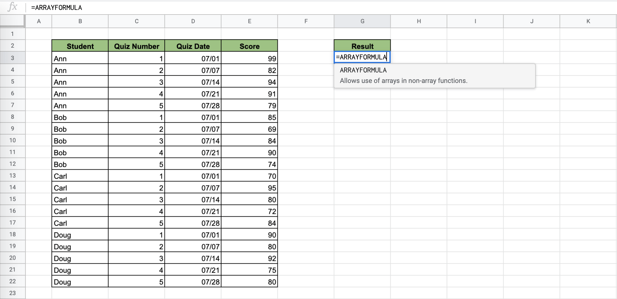
3. After that, type in the QUERY function. For now, just focus on the QUERY function and what’s inside it, and let the ARRAYFORMULA work its Google Sheet magic.

4. It’s time to fill in the first requirement, data. Add an open curly bracket to start this section. We want sorted columns of name and scores so that it’s easy to refer to it. In this example, we want the Alphabetical names of the students in order. We apply the data range B3:E. To sort the names, we pick column 1 and pick true for is_ascending. To sort the scores, we pick column 4 and pick false for is_ascending, since we’re already getting the highest 2 scores for each student.

5. The following IFERROR statement, you will note, uses the ROW and MATCH to find if the number of rows in the array minus the position of the matched item. This is part of the data range of the original QUERY statement. It’s advised that you follow this statement as is to avoid any errors, only adjusting the formula to your range and the desired data that you want. For example, we picked the ROW B3:B to pick the B column, and in MATCH picked the same data range from Step 4. Closeout your MATCH function with return_type 0. Close this data part in the original query function – don’t forget the closing curly brace!

This IFERROR statement is as follows:

=IFERROR(ROW(B3:B)-MATCH(QUERY(SORT(B3:E,1,true,4,false),"Select Col1"),QUERY(SORT(B3:E,1,true,4,false),"Select Col1"),0))

6. Add the query section of the QUERY function. Remember that we are interested in the Student name, and the top 2 scores. Write: “Select Col1, Col4, where Col5<4”, where Col1 is the names column, Col4 is the scores column. Wait – what does Col5 refer to then? Think about this: you are essentially creating a Col5 that displays your desired results. Now that we have to pick through those results as well, instead of accepting the number of values <3 (for two highest values), we need to use <4 because of that extra data.

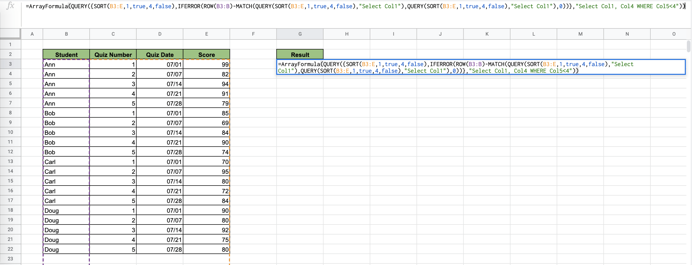
7. Close this out with a double parenthesis – because of ARRAYFORMULA – and you will see your list populate like magic!

And with that, you’re done! You can now use the above QUERY, SORT, ROW, and MATCH function to find the highest n values per group in a set. Create powerful spreadsheets with these formulas and more.

Get emails from us about Google Sheets.

Our goal this year is to create lots of rich, bite-sized tutorials for Google Sheets users like you. If you liked this one, you'll love what we are working on! Readers receive ✨ early access ✨ to new content. There will be no spam and you can unsubscribe at any time.

Subscribe