How to Use the SUMIF Function Horizontally in Google Sheets

The SUMIF function in Google Sheets is useful to get the sum of cells that meet the provided condition in a given range. In other words, the SUMIF function adds up cells that meet the given criteria.

In this guide, however, we will look at leveraging the SUMIF function to get the sum of cells horizontally. That is to say; you take the SUMIF criteria from the header row, not from the columns as you usually would.

There are a few things you should take note of while using the SUMIF function in Google Sheets:

• The SUMIF function requires (and accepts) just one condition only. Whereas the SUMIFS function allows you to input multiple conditions. 
• The conditions can be dates, texts, and/or numbers based.
• The function allows use of logical operators like (>,<,<>,=) and wildcards (*,?). For a comprehensive guide to using wildcards for the SUMIF function, refer to our article on the same here. 
• If the user doesn’t provide the third argument, the function will go ahead and sum up the values from the first argument by default.
• The function requires the user to input a range, and it should not be an array.
• Any text strings input as part of your conditions should be enclosed in quotation marks, unlike cell references, which shouldn’t.

Let’s take an example.

I have tabulated my monthly spending by expense type – bills, food, subscriptions, etc. Each group is listed under a month, and the months run from left to right on my sheet. I want to sum up the total spent on streaming services for the months of June and July. But since the table has been structured in a way where the months are adjacent to each other from left to right, the usual way to use SUMIF won’t help.

And this is where the additional capability of the function comes to my aid.

There are a couple of ways we can implement this in Google Sheets – one using the SUMIF function directly, and the other using an ARRAYFORMULA. We shall look at both of them with examples.

The Anatomy of the SUMIF Function

So the syntax (the way we write) of the SUMIF function is as follows:

=SUMIF(range, criteria, [sum_range])

Let’s look at the formula one term at a time and understand what each of them means:

• = the equal sign is how we start any function in Google Sheets. It is how Google Sheets understands that we are asking it to either do computation or use a function.
• SUMIF() is our SUMIF function. It gets the sum of cells that meet the provided conditions.
• range is the range of cells that we want to apply the criteria to.
• criteria is the condition that is used to decide which cells need to be summed up.
• [sum_range], an optional argument, contains numeric values that are to be summed up should the range entry meet the given criteria.

A Real Example of Using SUMIF Function

Take a look at the example below to see how SUMIF functions are used in Google Sheets:

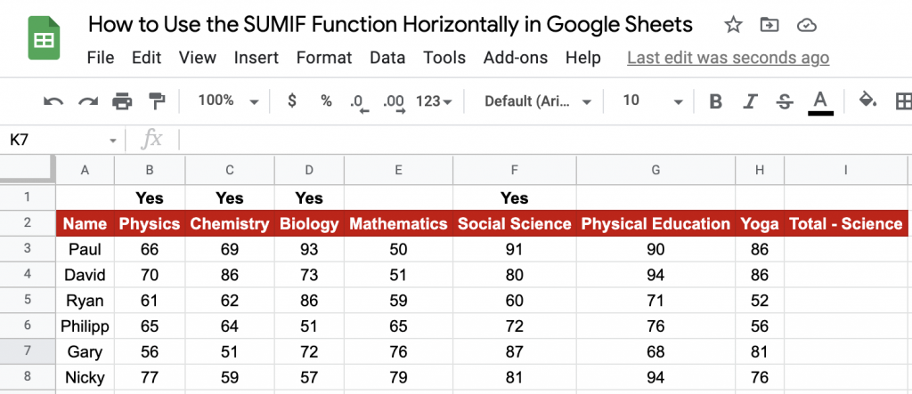
The above figures are marks secured by high school students in the city of Manchester. The objective here is to find the total marks obtained by each student in science subjects (which have been marked as Yes above the subject name).

As you can see below, I have obtained the total marks secured in science subjects for each student using the SUMIF function:

You may try changing the criteria and see how the result changes. Go ahead and make a copy of the spreadsheet using the link I have attached below:

Awesome! Let’s begin our SUMIF function in Google Sheets.

How to Use SUMIF Function in Google Sheets

1. Let’s see how to write your own SUMIF function, step-by-step. I have listed the unit sales of Home/Office Supplies across the entire year of 2020 at a nearby small retailer. The objective is to identify the total units sold for each of these items in the peak season when the schools and colleges reopen – the months of July, August and September. You will notice that I am using the header row itself here, unlike the additional row to specify the criteria as seen in the example earlier.

2. Now, simply click on any cell to make it the active cell. For this guide, I will be selecting N2, where I want to show my results.
3. Next, simply type the equal sign ‘=‘ to begin the function and then follow the function’s name, which is our ‘sumif‘ (or SUMIF, whichever works).
4. You should find that the auto-suggest box appears with our function of interest. Continue by entering the first opening bracket ‘(‘. If you get a huge box with text in it, simply hit the arrow in the top-right-hand corner of the box to minimize it. You should now see it as follows:

5. Now, the fun begins! Let’s give the required inputs to the function to get the total unit sales for each item for the peak sales season running from July through September:

6. Take note of how I’ve used SUM and ARRAYFORMULA to specify the months I want to be considered as the criteria. For a more comprehensive guide to using the ARRAYFORMULA, refer to our article on the same here.
7. Once you’ve entered the necessary values, or you’ve done what I did, make sure to close the brackets for all three functions, as shown below.

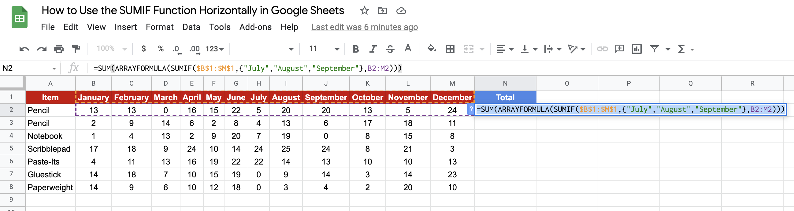
8. Finally, just hit your Enter key. You will notice that the results read 45 for colour pencils (which is row 2), 23 for lead pencils (which is row 3), 26 for notebooks and so on. This is because, based on the conditions we have given, the function only sums up values across three columns – the ones of July, August and September. 

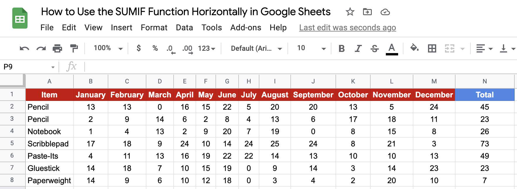
You can now see that we have the desired result – total sales units in the peak season for each item. That’s pretty much it. You have everything you need to get started with the SUMIFfunction on Google Sheets. I recommend experimenting with the SUMIFfunction, combining it with the numerous Google Sheets formulas available, and seeing what you can come up with. 🙂

Get emails from us about Google Sheets.

Our goal this year is to create lots of rich, bite-sized tutorials for Google Sheets users like you. If you liked this one, you'll love what we are working on! Readers receive ✨ early access ✨ to new content.

Subscribe