This guide will discuss how to filter the last status change rows in Google Sheets.
We will show you how to extract specific values from the data set that meet the specified conditions or criteria.
Google Sheets has a powerful and useful FILTERfunction that allows filtering data. But no standalone function allows us to filter the last status change rows in Google Sheets.
Hence, we will be using a formula that is a combination of the FILTER function and SORTN function. This function is used to sort a range of data and only return specific values from the sorted result.
Let’s consider this example.
Suppose you are working in the post office. You get hundreds of packages each day to keep track of. So you highlighted the latest value change rows of the delivered packages. But the number of packages is too much to keep up with and is making it difficult to quickly identify the statuses.
Hence, you decided to filter the last status change rows. This way you can easily see the status of the packages since the unnecessary values have been filtered out. And you can only see the packages that are successfully delivered.
Learning how to filter the last status change rows in Google Sheets will be helpful in cases like the one above and in many others. Now let’s move on and discuss a real example of filtering the last status change rows in your data set.
A Real Example of Filtering Last Status Change Rows in Google Sheets
Since you are filtering the last status change rows, it means you are done highlighting the latest value change. First, let’s see what your data set would look like before filtering.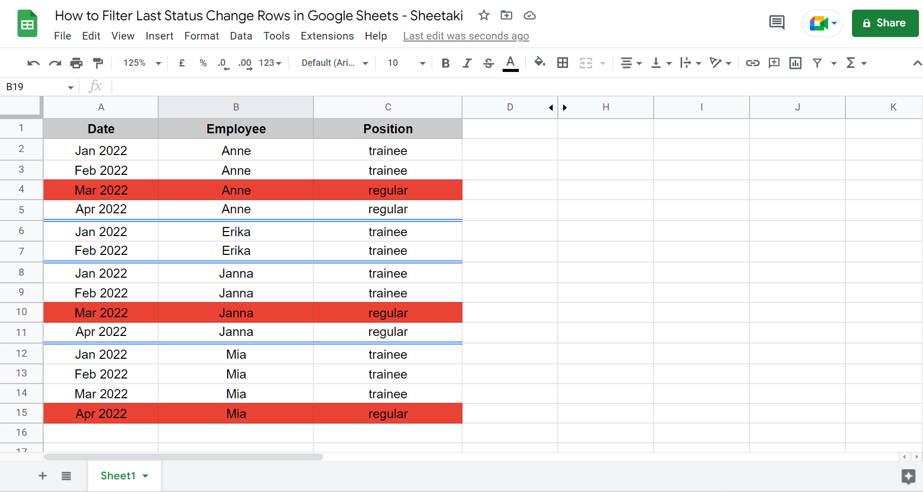
The last status change row is highlighted in red. Anne and Janna became regulars in March 2022, while Mia became a regular employee in April 2022, and Erika did not change.
To filter the last status change rows, you need to combine the columns. Usually, the ARRAYFORMULA function would be used. But in this case, you will use a combination of the TRANSPOSE and QUERY functions.
First, you need to eliminate the duplicated rows based on Employee and Position, which are columns B and C, respectively. Furthermore, you will eliminate again the duplicated rows based on Employee, which is column B.
So this will leave you with only one unique record from each group. That is one employee from each group. After, you need to identify the last status change rows. Finally, you use the filter formula ‘=filter(A2:C,U2:U*V2:V>1)‘ to get filter the last status change rows.
Essentially, it is a process of eliminating duplicates using the SORTN function. Then, with the use of the FILTER function, only the last status change rows will remain. 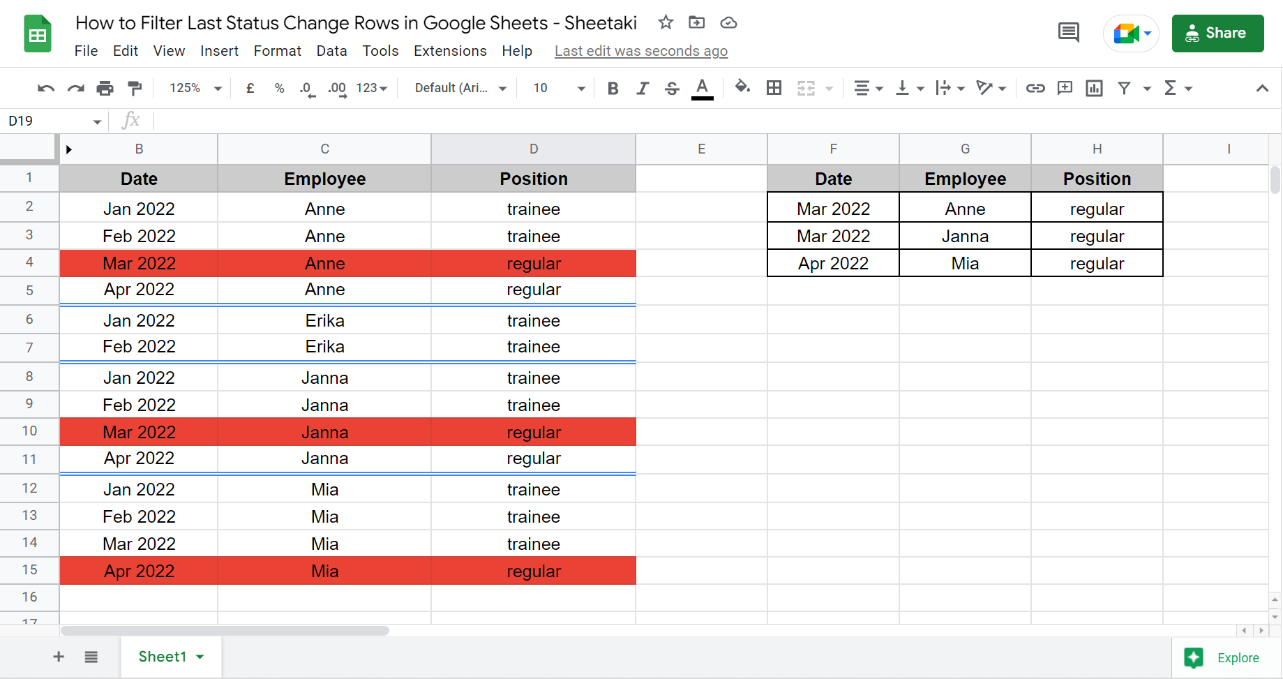
You can make your own copy of the spreadsheet above using the link attached below.
Since you now have a general idea of what it would look like to filter the last status change rows in Google Sheets, let’s move on!
How to Filter Last Status Change Rows in Google Sheets
In this section, you will learn how to filer the last status change rows in Google Sheets.
1. First, eliminate the duplicate rows. We will base the duplicated rows on columns B and C, which are the Employee and Position. ‘=sort(sortn({B2:D,row(B2:B)},8^8,2,transpose(query(transpose(C2:D),,8^8)),1),2,0,4,1)’. Press enter to show results.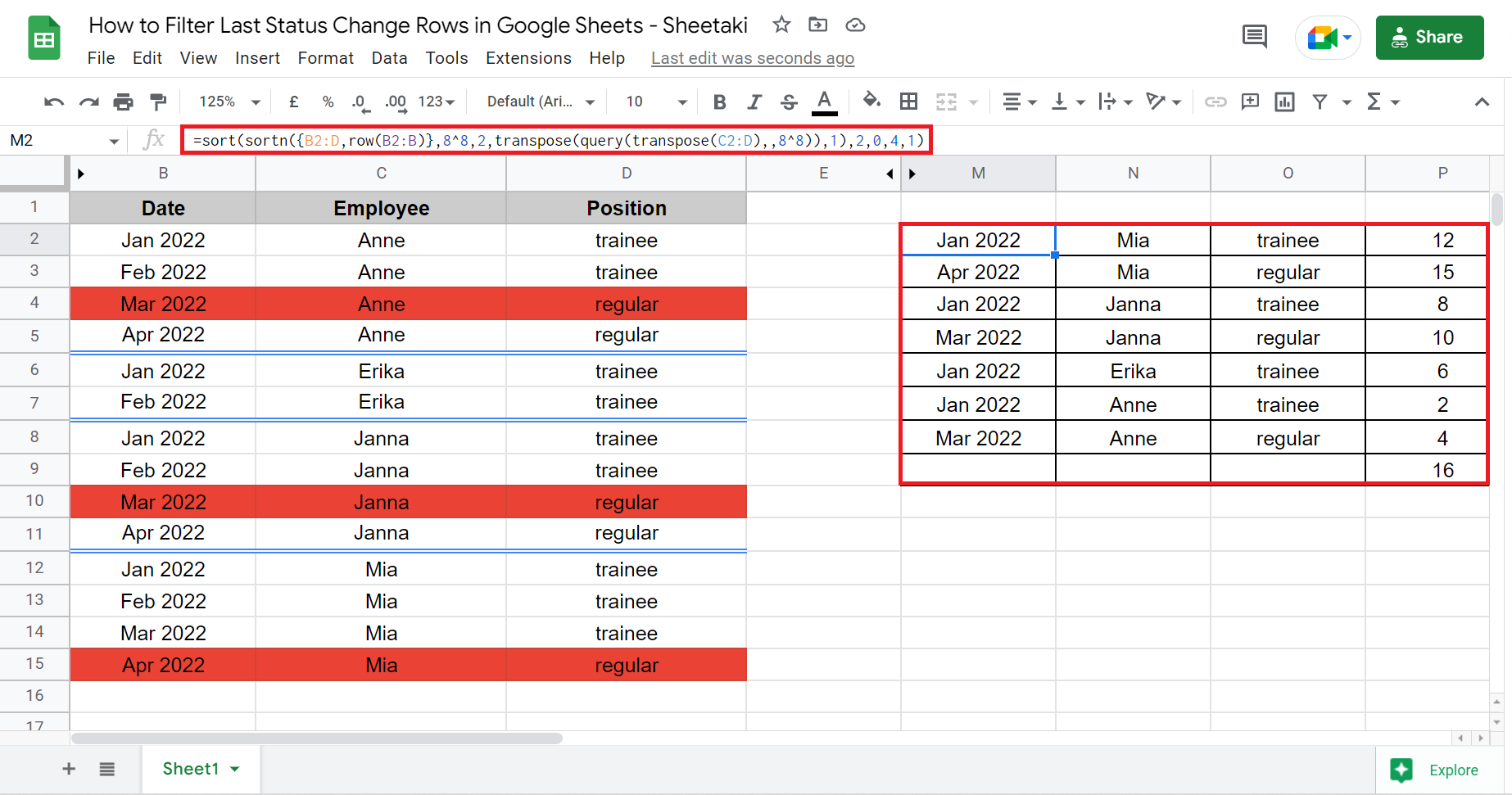
This formula will sort the data and return it without the duplicated rows. On the right side of the table, those are the corresponding row numbers.
2. Second, you need to further eliminate the duplicated rows based on Employee, which in this case is column I. Type this formula ‘=array_constrain(sortn(sort(sortn({B2:D,row(B2:B)},8^8,2,transpose(query(transpose(C2:D),,8^8)),1),4,0,2,1),8^8,2,2,1),8^8,3)’. Press Enter to show results.
So this formula will sort the data in the table from the first step and return another table that only has one unique record for each employee. That is only one row from each employee.
3. Next, you need to identify the last status change rows. To do this, type this formula ‘=ArrayFormula(IFNA(vlookup(transpose(query(transpose(B2:D),,8^8)),transpose(query(transpose(array_constrain(sortn(sort(sortn({B2:D,row(B2:B)},8^8,2,transpose(query(transpose(C2:D),,8^8)),1),4,0,2,1),8^8,2,2,1),8^8,3)),,8^8)),1,0)))’.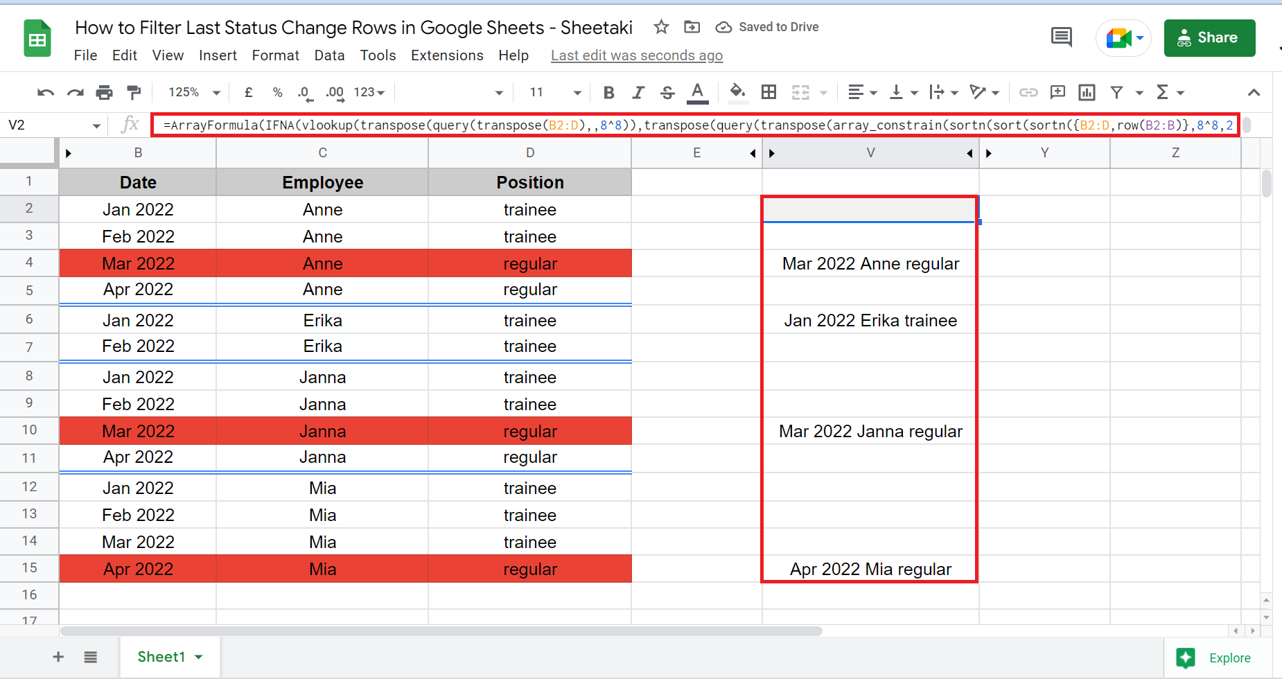
4. Then, you need to convert the last status change rows to 1 and the blank cells to 0. To do this, type in ‘=ArrayFormula(--istext(IFNA(vlookup(transpose(query(transpose(B2:D),,8^8)),transpose(query(transpose(array_constrain(sortn(sort(sortn({B2:D,row(B2:B)},8^8,2,transpose(query(transpose(C2:D),,8^8)),1),4,0,2,1),8^8,2,2,1),8^8,3)),,8^8)),1,0))))’.
5. Also, you need to have the sequence of Employee or column B. This will help find the last status change rows. So type in ‘=ArrayFormula(countifs(row(B2:B),”<=”&row(B2:B),C2:C,C2:C))’. Press enter to show results.
6. Lastly, you need to create a separate table with the change rows. To do this, type in ‘=filter(B2:D,--istext(IFNA(vlookup(transpose(query(transpose(B2:D),,8^8)),transpose(query(transpose(array_constrain(sortn(sort(sortn({B2:D,row(B2:B)},8^8,2,transpose(query(transpose(C2:D),,8^8)),1),4,0,2,1),8^8,2,2,1),8^8,3)),,8^8)),1,0)))*countifs(row(B2:B),"<="&row(B2:B),C2:C,C2:C)>1)’ in a blank cell next to the data set.
7. And tada! Here is the final output of filtering the last status change rows in Google Sheets.
8. When you have multiple columns, you only need to change the range in the formula. For instance, you have another column for the departments of each employee.
You can use this formula, ‘=filter(B2:E,--istext(IFNA(vlookup(transpose(query(transpose(B2:E),,8^8)),transpose(query(transpose(array_constrain(sortn(sort(sortn({B2:E,row(B2:B)},8^8,2,transpose(query(transpose(C2:D),,8^8)),1),5,0,2,1),8^8,2,2,1),8^8,4)),,8^8)),1,0)))*countifs(row(B2:B),"<="&row(B2:B),C2:C,C2:C)>1)’. Press enter to show results.
And it will return a table similar to the previous step. But now, you have an additional table that includes column E, which is the last status change rows of the department.
That’s pretty much it! You have learned how to filter the last status change rows in Google Sheets. So you can apply this to situations where you need to identify specific values, making your work more efficient.
Are you interested in learning more about what Google Sheets can do? Make sure to subscribe to our newsletter to be the first to know about the latest guides and tutorials from us.