How to Use FILTER Function in Google Sheets [Step-By-Step]

The FILTER function in Google Sheets is useful to filter and return the rows or columns in a range that meet the criteria we specify.

The Anatomy of the FILTER Function
A Real Example of Using FILTER Function
How to Use FILTER Function in Google Sheets

Filtering is one of the most powerful and most important features there is in Google Sheets.

The FILTER function is used to filter the rows of a given range by the conditions of our choosing. We can filter based on one or more conditions.

Let’s take an example.

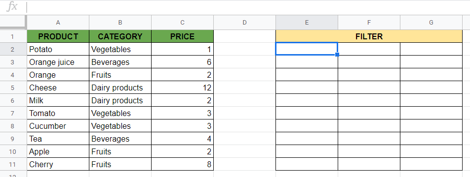
Say we have a list of food products. 🍅🧀

We would like to retrieve all products below a certain price as well as values that are in a specific category like vegetables, dairy products, etc.

So how can we do that?

It’s simple. The FILTER function only needs the range where we are filtering and the conditions that we need.

As a result, we get a new data set which only shows the rows/columns from the original data set that meets the conditions set in the formula.

Now before we dive into some real examples, let’s understand how the FILTER function in Google Sheets works.

The Anatomy of the FILTER Function

The syntax of a function specifies how we should use the function. For the FILTER function, the syntax looks like this:

=FILTER(range, condition1, [condition2, ...])

Let’s break this function down and understand what each of the terms mean:

= the equal sign is how we start every function in Google Sheets.
FILTER is our function. We will have to add the following variables into it for it to work.
range is the data to be sorted.
condition1 is a column or row containing TRUE or FALSE values corresponding to a selected column or row of the range. It can be an array formula evaluating to TRUE or FALSE too. At least one condition is required to use in the function.
condition2, ... are additional conditions where their use is optional. You may set more than one conditions that should be checked.

⚠️ A Few Notes to Make Your FILTER Function Work Perfectly

As a condition, you can define any formula, that returns a TRUE or FALSE result. You may use simple operators (=, <, >), but even complicated expressions with several functions in it.
You are not allowed to use both row and column conditions in the same formula. To filter both rows and columns, you can use the return value of one FILTER function as the range in another.
The range that you want to filter can be a single column or multiple columns.
The ranges that are used in the condition1, condition2 … variables must be single columns.
Each condition should be of the same size as the range. In other words, the source range and the range for the condition must contain the same number of rows/columns.
You have to make sure that there is enough empty area for your filter results. Before writing the function, select a clear area in your sheets where you can put your results.

Having now gained some brief insight into FILTER functions work, let’s jump right into some examples where we can write our own FILTER functions.

A Real Example of Using FILTER Function

Have a look at the examples below to understand how to use the FILTER function in Google Sheets.

FILTER Function with One Condition

In the first example, we defined one condition to filter by.

Using FILTER with one condition

We have the list of food products, and we wanted to filter those that are in the “Dairy products” category.

The following formula will do the job:

=FILTER(A2:C11,B2:B11="Dairy products")

As a result, we get a new table with the filtered products that meet our criteria.

Here is what this example does:

We selected a cell where we wanted to put the first result of our filtered new data set. Here we wrote the formula in cell E2.
We wrote a FILTER function with two variables. The first variable is the range, that is all the data set we have in the range A2:C11.
Then, we added the only criteria, called condition1. As we are filtering for categories, the range of the condition is B2:B11 where the categories are.
To filter only the dairy products, we used an equality check as our TRUE or FALSE condition. We added =”Dairy products” to our condition to check whether the cells in the range B2:B11 match this text.
We got our filtered products that match the condition. As you can see, the two products (Cheese and Milk) are the only dairy products in the original list.

Super easy, right?

You can make a copy of the spreadsheet using the link I have attached below and have a go at it yourself:

Make a copy of example spreadsheet

FILTER Function with Multiple Conditions

You can understand from the syntax of the FILTER function that it is possible to filter by multiple (two or more) criteria.

Let’s use the same food products and say we want to retrieve the products which are fruits and their price is below 5.

Using FILTER with multiple conditions

The FILTER function with more conditions is as follows:

=FILTER(A2:C11,C2:C11<5,B2:B11="Fruits")

It works exactly the same way as the first example.

The difference is that we added two conditions as variables:

C2:C11 < 5 means that we filtered the products by their price, and only kept those that have a price lower than 5.
B2:B11=”Fruits” means that we checked for the Category column and filtered the products that have “Fruits” in it.

The filtered results meet both of the criteria we set, so their prices are below 5, and they are in the “Fruits” category.

We can add even more conditions. The only important thing is that these conditions should be TRUE or FALSE expressions, and the size of the ranges should match the size of the original range.

How to Use FILTER Function in Google Sheets

Let’s begin writing your own FILTER function step-by-step.

Before starting it, you need to decide where you would like to put your filtered data. For this guide, we will make sure that the area E2:F11 is empty before starting to work with the FILTER function:

Selecting Active Cell