The IMPORTFEED function in Google Sheets is useful if you want to import an RSS or ATOM feed into your worksheet.
Meaning, the IMPORTFEED function allows you to keep track of new blog posts or news items on your favorite website.
Table of Contents
The rules for using the IMPORTFEED function in Google Sheets are as follows:
- The first (url) and second arguments ([query]) of the IMPORTFEED function need to be enclosed with quotation marks or can be a cell reference.
- The higher the number of results from the website, the longer it may take to finish the data import.
- The IMPORTFEED function returns arrays of information
- The IMPORTFEED function will return a #REF! Error if the expected range of results isn’t clear for any values.
- The second ([query]), third ([headers]), and fourth arguments (num_items) are optional. If no values are passed to these arguments, the IMPORTFEED function will assign the default values for each.
- There are only expected values for the second argument ([query]) and the function will return the #VALUE! error if it isn’t one of them.
Let’s take an example.
Kris would like to be updated on the blog posts of her favorite website, Sheetaki.com. Aside from being subscribed, she also likes to have a Google Sheet file that has the lists of the most recent blog posts made by the website.
With the help of the IMPORTFEED function, she was able to create a Google Sheet file that pulls the most recent article being published on Sheetaki.com.
See the file she created below:

The IMPORTFEED helps Kris to get a glimpse and track the most recent contents of her favorite website.
Watch out for a more advanced tutorial and examples on how you can use the IMPORTFEED function in the coming weeks. Be sure to subscribe to be notified.
Perfect! Let’s begin getting to know more about our IMPORTFEED function in Google Sheets.
The Anatomy of the IMPORTFEED Function
So the syntax (the way we write) the IMPORTFEED function is as follows:
=IMPORTFEED(url, [query], [headers], [num_items])
Let’s dissect this thing and understand what each of these terms means:
- = the equal sign is just how we start any function in Google Sheets. It is how Google Sheets understand that we are asking it to either do computation or use a function.
- IMPORTFEED() this is our IMPORTFEED function. It allows you to easily import an RSS or ATOM feed from a feed source.
- url is the address (uniform resource locator) of the feed file, from which you’re importing data.
- [query] is an optional argument that specifies what data to fetch or import from the url.
- [headers] is also an optional argument that tells the function whether we would want header values or not.
- [num_items] is an optional argument as well which limits the number of contents the function will return.
A Real Example of Using IMPORTFEED Function
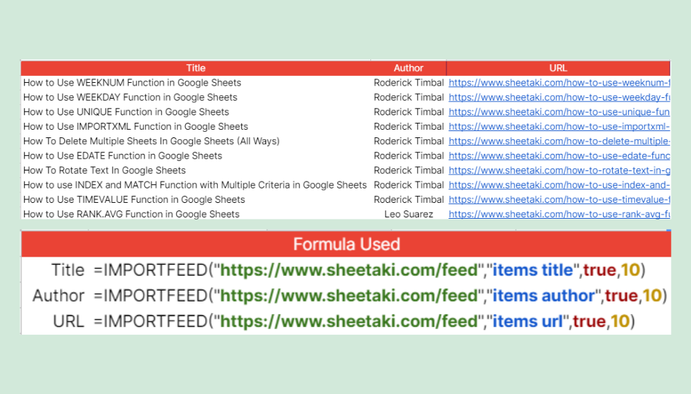
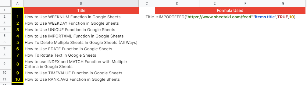
Let’s take a look at the file that Kris made below to see how the IMPORTFEED function is used in Google Sheets.
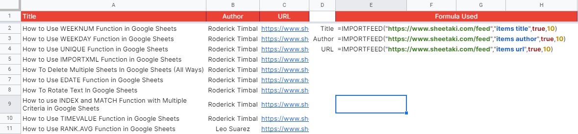
In column A, she imported the titles of the recent blog posts on the Sheetaki website.
Let’s analyze how the IMPORTFEED pulled this information from that website.
Take a look at the formula used below:
=IMPORTFEED(“https://www.sheetaki.com/feed”,”items title”,true,10)
The first argument is the RSS or ATOM feed URL of the website you want to pull the information from. In our example above, it is ‘https://www.sheetaki.com/feed’ and is enclosed with quotation marks.
But, how do we get the RSS or ATOM feed URL of a specific website?
In most cases, you can append ‘/feed’ to the domain of a website to get its feed file. So, in our example above, ‘https://www.sheetaki.com’ is the domain, and we put ‘/feed’ at the end of it. Hence, our first argument is ‘https://www.sheetaki.com/feed’.
Alternatively, to find the RSS feed of Sheetaki.com, just do a right-click anywhere on the screen and click on “View Page Source” (control + u in Chrome).

Search for the word ‘feed’ to find the feed URL of that site.
![]()
This URL can be used as the first argument for the IMPORTFEED function.
Let’s move to the second argument used in our example above, ‘items title’.
It simply means that we are instructing the IMPORTFEED function to import or return the titles of the posts on our source website.

The information above corresponds to the titles of the most recent posts on Sheetaki.com.

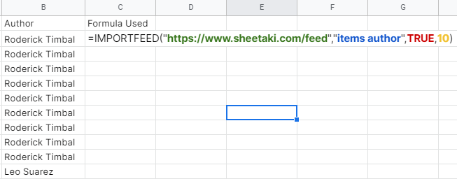
The value for the 2nd argument can also be the author (items author), summary (items summary), or the URL (items url) of the post.
See the examples below:

We passed the values ‘items author’ and ‘items url’ to our IMPORTFEED functions to return the names of the authors and the URLs of the recent posts in Sheetaki.com.
The 3rd argument passed to our IMPORTFEED function above is the Boolean value TRUE. This means that we wanted the IMPORTFEED function to include the header title of the information we are importing.
See the header title in cell A1 below:

If we are to pass FALSE as the third argument, it wouldn’t include the header title. Please see the sample below:

Notice that in cells A1, B1, and C1, the values are already the information of the first content. You will have to insert a row above so that you can manually put the header titles for each information.
For our last argument, it limits the function to return the number of items.
In our example above, we passed the value 10 as the 4th argument, which told the IMPORTFEED function to only show the 10 most recent posts on the website.
If we will change the 4th argument to 5, it would only show 5 items:

You may make a copy of the spreadsheet using the link I have attached below.
How to Use IMPORTFEDD Function in Google Sheets
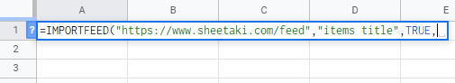
- Click on any cell to make it the active cell. For this guide, I will be selecting A1, where I want to show the imported information.

- Next, type the equal sign ‘=‘ to begin the function and then follow it with the name of the function, which is our ‘importfeed‘ (or ‘IMPORTFEED‘, not case sensitive like our other functions).

- Type open parenthesis ‘(‘ or simply hit Tab key to let you use that function.

- Now the exciting part! Let’s give our function its first argument, the url. Type in the quotation mark (“) and follow it with the website feed URL. In this case, I will be using ‘https://www.sheetaki.com/feed’. Don’t forget to close it with another quotation mark (“).

- To let the Google sheet know that we’re done typing our first argument, we should now type in the delimiter or the character that separates each argument on a function. In this case, type comma ‘,’.

- Type in our second argument, which is the optional argument [query]. Type in quotation mark (“) and follow it with ‘items title’. Don’t forget to close it with another quotation mark (“).

- Before we type in our third argument, make sure to end the second argument with our delimiter. Type in comma (,).

- Now, let’s pass the third argument. Since we want our IMPORTFEED to include the header title of the information, type in ‘TRUE’ and follow it with another delimiter. No need to enclose the Boolean value with the quotation mark.
- For the fourth argument, type in ‘10’ for the function to return 10 content titles.

- Finally, hit your Enter or Tab key. Cell A1:A11 will now show you the resulting array of information or the return value of the IMPORTFEED function, which are the 10 content titles from our website feed source.

- Now, let’s extract the author of these content titles.
- On cell B1, repeat steps 1 to 10. Only this time, for step 6, type in ‘items author’.

- Then, hit your Enter or Tab key. Cell B1:B11 will now show you the 10 content authors of the 10 most recent posts in Sheetaki.com.
That’s pretty much it. You can now use the IMPORTFEED function in Google Sheets together with the other numerous Google Sheets formulas to create even more powerful formulas that can make your life much easier.