How to Use TRIM Function with SPLIT in Google Sheets

The TRIM function in Google Sheets is a nifty little tool that is especially useful for cleaning up those unnecessary spaces in your spreadsheets. Here, we will be learning how to use TRIM function with SPLIT in Google Sheets.

The TRIM function one of many built-in functions in Google Sheets that are designed to both clean up the data you put into your spreadsheet.

I’m sure you have encountered data in Google Sheets with the odd leading spaces that throws the alignment off, the unnoticed trailing spaces when you copy the data externally or the occasional double space from a typo. 😱

In this guide, we will be teaching you not only how to use the TRIM Function but also how to combine it with the SPLIT Function. Before we begin, however, if you would like to learn more about the SPLIT Function, you can find a detailed guide here.

Now, imagine that you were planning a birthday party and created a public Google Sheets for the invitees to RSVP and provide their details. Unfortunately, as mentioned above, typos happen, and you notice that the spreadsheet has several unnecessary spaces in the data.

So how do we remove these spaces?

Easy. 😉 We use the TRIM format that automatically detects these spaces and removes them summarily.

Now, let’s move on to the next section to see how to use the TRIM function in Google Sheets.

 

 

How to Use the TRIM Function

There are two ways you can use this function. The first of which is already built into the Google Sheets menu.

The first method is to simply clean up any unnecessary spaces in your selected data using the Google Sheets menu. This can be accomplished by accessing the Google Sheets Menu>Data and clicking on “Trim Whitespace”.

 

 

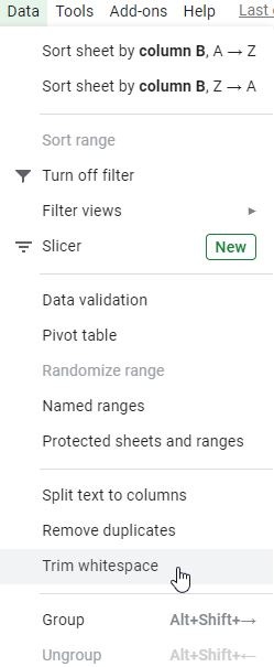
At this point, Google Sheets will instantly go through the text in every selected cell and look for any spaces that occur at the beginning of the text, after the end of the text as well as any whitespaces other than the single space between words.

Keep in mind that this directly overwrites the data in the selected cells.

Now, the second method of using the TRIM function is to use this formula:

=TRIM(text)

Let’s break down this function:

• = is the equal sign and it is how we start any function in Google Sheets.
• TRIM() will be our function. For it to be operational, we need to add the text attribute inside the parenthesis.
• text is the cell or range of cells that you would like to apply the TRIM function on.

Now that you have an idea on how the TRIM function works, we’ll move on to some examples in the next section.

 

 

A Real Example of Using the TRIM Function

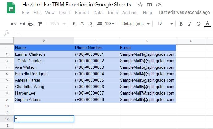
Using our initial example of a spreadsheet tracking a birthday party’s guest information, we will be using the below data to demonstrate how to use the TRIM function.

 

As you can see, we have several unfortunate typos in the data.

To clean this up, first, highlight the entire “Name” column.

Next, access the Google Sheets Menu>Data and click on the TRIM function.

Voila!🎉🎉🎉 Google Sheets has now removed all those annoying additional white spaces in the data.

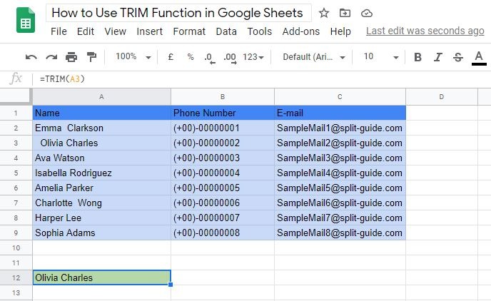
Alternatively, if you prefer to use the function, select the cell where you would like the cleaned data to be displayed. For this example, we are going to input our function in cell D2.

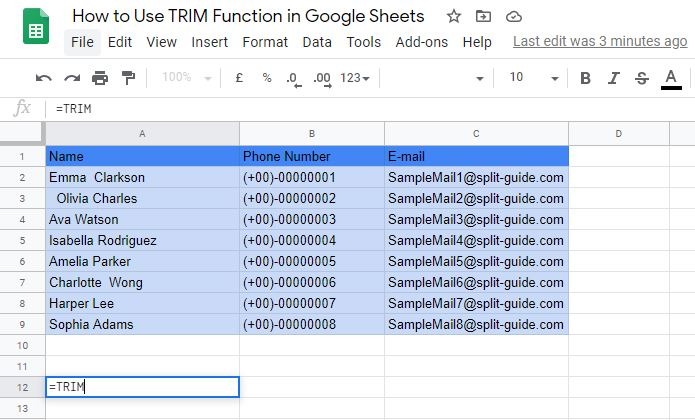
Next, we input the syntax from the previous section “=TRIM(text)”.

Thirdly, for this example, we will input cell A2 as the text attribute.

Finally, hit the Enter key and Google Sheets will have removed the extra white space in between Emma Clarkson’s name.

Simple right?

You can make a copy of the spreadsheet using the link I have attached below

 

 

A Real Example of Using the TRIM Function With SPLIT

Before we begin to learn how to use the TRIM function with SPLIT in Google Sheets, let’s do a quick recap of the SPLIT function. In Google sheets, the SPLIT function is used to separate text in a cell by a common delimiter into separate columns.

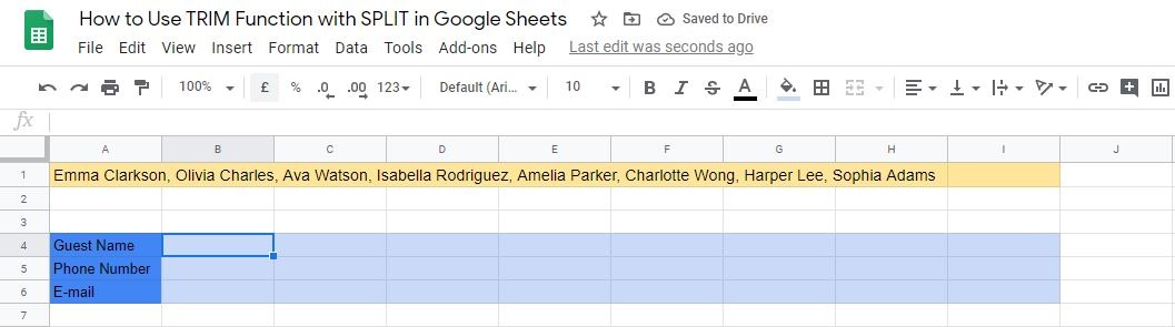
A more relevant example would be to imagine that the party’s guest list was sent to you in this format: “Emma Clarkson, Olivia Charles, Ava Watson, Isabella Rodriguez, Amelia Parker, Charlotte Wong, Harper Lee, Sophia Adams”

Normally, it would take a lot of time and effort just to put each individual name into their respective cells. Now, imagine if the guest list numbered in the hundreds. That’s where the SPLIT function comes in. By using the comma symbol “,” as the delimiter, the SPLIT function will separate each name into a separate column saving you a lot of time.

Again, if you would like to learn the SPLIT function in more detail, you can find Sheetaki’s step-by-step guide here. 

The data below will be used for this example.

 

As mentioned above, the first step in handling this data would be to use the SPLIT function to separate the names into separate cells.

For this example, we will be  using the SPLIT formula

=SPLIT(A1, “,”)

As expected, Google Sheets splits the names into cells B4 to I4. However, as you can see, after the splitting, the data in cells C4 – I4 all have a whitespace at the beginning of the data.

This is due to the fact that the delimiter does not include the whitespace behind each comma. To remove these whitespaces, you would normally be able to use the TRIM function together with the SPLIT function.

However, if you try to use the formula =TRIM(SPLIT(A1,”,”)), this happens:

 

You end up with just the first name, “Emma Clarkson” in cell B4 with cells C4 – I4 completely empty. This happens because when you use the SPLIT function, the result is an array and not just a single cell. As the TRIM Function only works on a single cell at a time, only the first cell in the array is processed and displayed by the TRIM function.

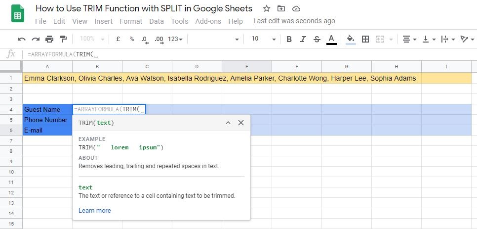
That is why we need to utilize the =ARRAYFORMULA() function together with our existing formula. The ARRAYFORMULA function allows us to use non-array functions like TRIM with arrays. For those of you not familiar with how to use the ARRAYFORMULA function, you can check out our detailed guide here.

Our new formula becomes

=ARRAYFORMULA(TRIM(SPLIT(A1,”,”)))

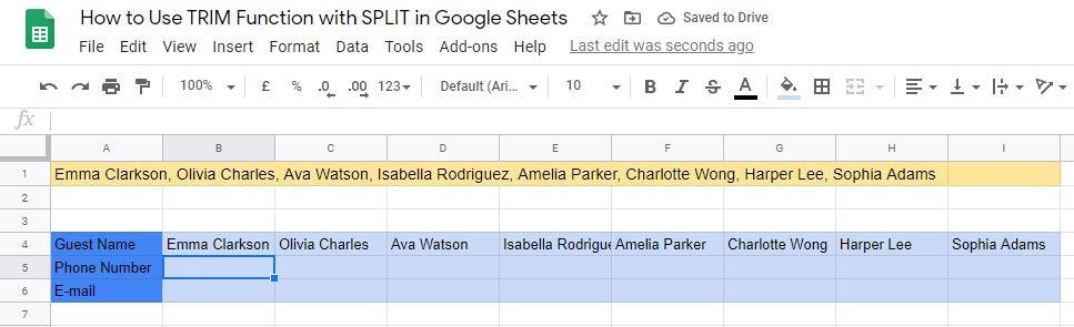
Once you hit enter, you will see that the names are split correctly and the TRIM Function has removed all the leading whitespaces.

It might sound a little complicated but don’t worry, we will provide a step to step guide in the next section. Before that, if you’d like to try the formula yourself, you can grab a copy of the example data from the link below:

 

 

 

How to Use the TRIM Function in Google Sheets

1. First, click on an empty cell to activate it.

 

2. Next, type the equals sign “=” to let Google Sheets know that you are going to input a formula.

 

3. Thirdly, you want to type TRIM to use the function.

 

4. Remember to key in an open parenthesis “(“ here before inputting the text.

 

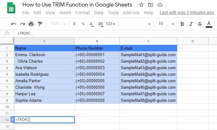
5. For the text attribute, we can select the cell A3 with our cursor.

 

6. Alternatively, you can also type it in manually.

 

7. Hit the Enter key, and all the unnecessary whitespaces will be removed.

---

How to Use the TRIM Function with SPLIT in Google Sheets

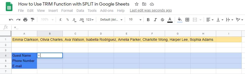
1. First, click on an empty cell to activate it

 

2. Next, type the equals sign “=” to let Google Sheets know that you are going to input a formula

 

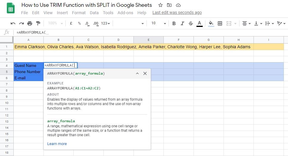
3. Here, you will input ARRAYFORMULA as the first function we will be using in this formula.

 

4. Input the first open parenthesis “(“.

 

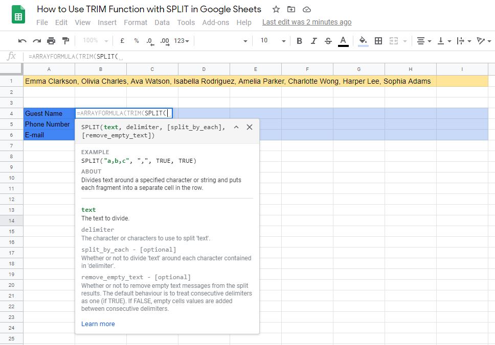
5. Follow that with the second function, TRIM, and another open parenthesis “(“.

 

6. Here, in place of the text attribute, we will input our third and final function in the formula, SPLIT.

 

7. Input yet another open parenthesis “(“ and Google Sheets will display the attributes that you need to input next for the SPLIT function to work.

 

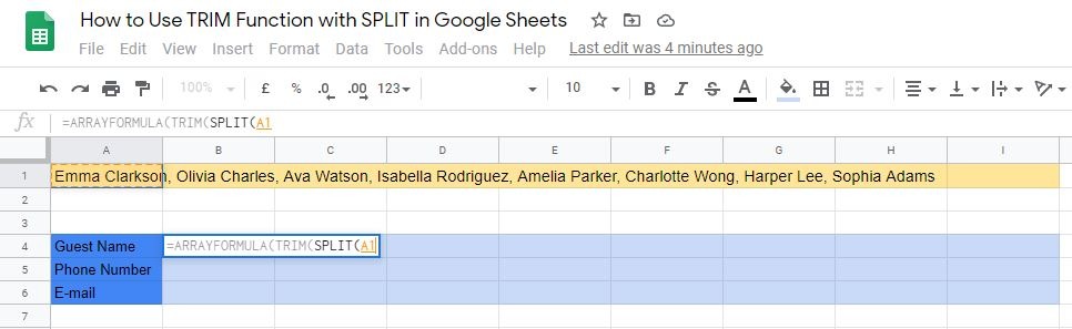
8. Next, we need to input the text attribute of the SPLIT function. You can just click on the cell containing the data (A1) you would like to split or key it in manually.

 

9. Remember to add a comma symbol “,” here before you enter the delimiter attribute.

 

10. For this example, we will be splitting the text using the commas “,” in the text as the delimiter attribute. Make sure to always wrap the delimiter value with double quotation marks “”.

 

11. Hit the Enter key and the TRIM function will have separated the text while the TRIM function will have removed any of the leading whitespaces in the array’s data.

 

And that’s it! Great job for completing the guide 👍. You can now use the TRIM function with SPLIT in order to help you with your day-to-day Google Sheets work. You can even combine the TRIM function with other numerous Google Sheets formulas to make your life even easier!