The AVERAGEIF function in Google Sheets is useful if you want to get the average of a row or column, given that it meets the desired criteria.
Table of Contents
The AVERAGEIF function does this simply by taking it as one and using it right away. Meaning, there is no need to combine the AVERAGE and IF functions.
The way we use the AVERAGEIF function in Google Sheets is almost similar to how we use the AVERAGE function. The only difference is just that, with AVERAGEIF, we are working with given conditions.
Let’s take an example to understand this clearly.
Say we run a Math session with ten students. These students come from different levels — level 1 to level 5. We want to check the average of students in level 3.
So how do we do that?
Easy. We can use our AVERAGEIF function to calculate for the average, given our condition, which is only level 3 students. We will now supply our function with the necessary attributes to make it work perfectly.
Ultimately, the AVERAGEIF function will output to the average grade of students in level 3.
You can surely do a lot of things with this AVERAGEIF function. For variety, we can also check the average population of men and women, an age group, or anything depending on your desired condition.
See how simple that is?
Now, let’s dive into real-business examples where we will deal with actual values and textual strings and see how we can write our own AVERAGEIF function in Google Sheets to compute those data.
The Anatomy of the AVERAGEIF Function
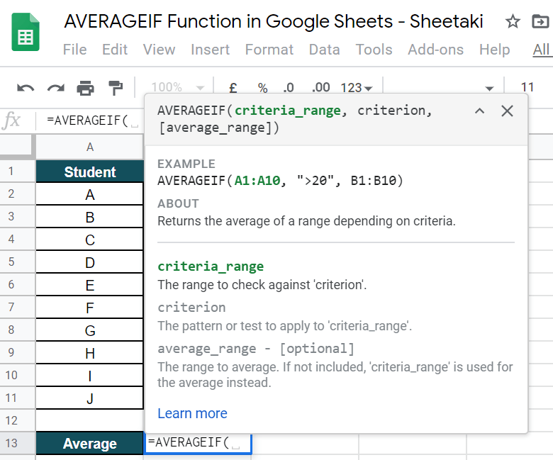
So the syntax (or how we write) the AVERAGEIF function is as follows:
=AVERAGEIF(criteria_range, criterion, [average_range])
Let’s break this syntax down into pieces to understand what each terminology means:
=the equal sign is how we start any function in Google Sheets.AVERAGEIF()is our function. All we need to do now is to add thecriteria_range,criterion, andaverage_range(optional) attributes to make our function work seamlessly.criteria_rangeis the range where the values that we want to check are located.criterionis the condition or test that we would like to meet.[average_range]is an optional address to the range that theAVERAGEIFconsiders. If in case we do not want to use this, theAVERAGEIFfunction will average thecriteria_range.
⚠️ Now a note before writing your own AVERAGEIF formula.
- We have a total of 6 comparison operators to choose from, depending on how we want to state our condition, and they are the following:
- = (equals)
- <> (not equal to)
- > (greater than)
- < (less than)
- >= (greater than or equal to)
- <= (less than or equal to)
It may look so confusing at this moment, but we’ll help you iron out important details and give clear examples and easy guide. We will go through the step-by-step process of using the AVERAGEIF function in Google Sheets.
A Real Example of Using AVERAGEIF Function
To see how AVERAGEIF function is used in Google Sheets, have a look at the example below.

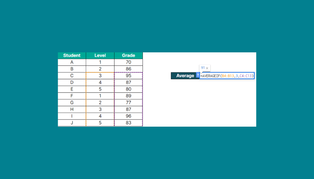
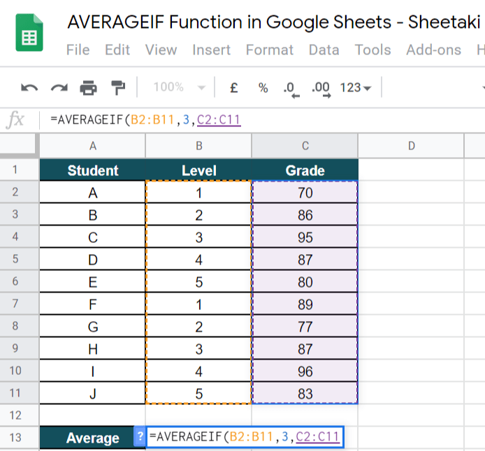
As you can see in the example above, the AVERAGEIF function is used to calculate for the average grade of Level 3 students. The function yields an answer of 91, the average of Students C and H. The function is as follows:
=AVERAGEIF(B2:B11,"3",C2:C11)
Here’s what this example does:
- We have actively selected an empty cell and used the
AVERAGEIFfunction to calculate the average grade of only level 3 students. The result will be shown in cell B13. - We selected column B as our criteria_range. This is where the condition, ‘level 3’ is checked.
- Next, we will add 3. This signifies the condition, ‘level 3’. At this point, we may opt not to include a comparison operator because, for this example, we only want to check one condition – if not level 3, then it will automatically disregard. If in case, you want to add an operator, then it would be “=3”.
- After that, we will now add the range to average. For this guide, we selected the range, C2:C11.
Super easy, right?
Feel free to make a copy of the spreadsheet using the link I have attached below and try it for yourself:
Let’s begin writing our own AVERAGEIF function in Google Sheets.
How to Use AVERAGEIF Function in Google Sheets
- Click on an empty cell to make it active. This is where we want to write our answer. For this guide, I selected cell B13.

- Next, simply start with an equal sign (=), followed by our function, AVERAGEIF, then, an open parenthesis “(“.

- Now, wait for the pop-up message as this will serve as our extra guide.
- After that, we will select the range B2:B11. In this cell lies the levels of students. This is the range to check against our criterion.
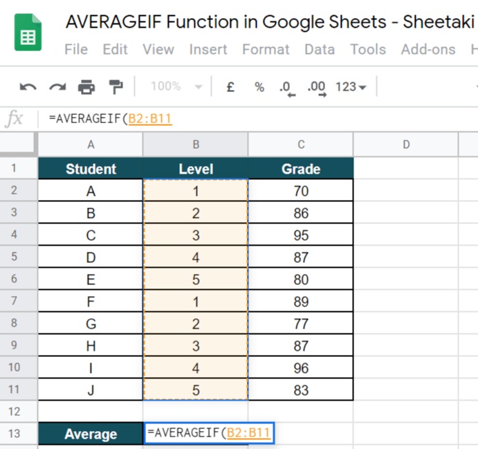
- Then, we now add our criterion, which is 3. No need to add a comparison operator because we just want to check those equal to 3, or an exact match – not more or less.

- After adding our criterion, we now select the range to average, and that is found in column C. Let’s select C2:C11.
- Close the formula with a close parenthesis, “)“
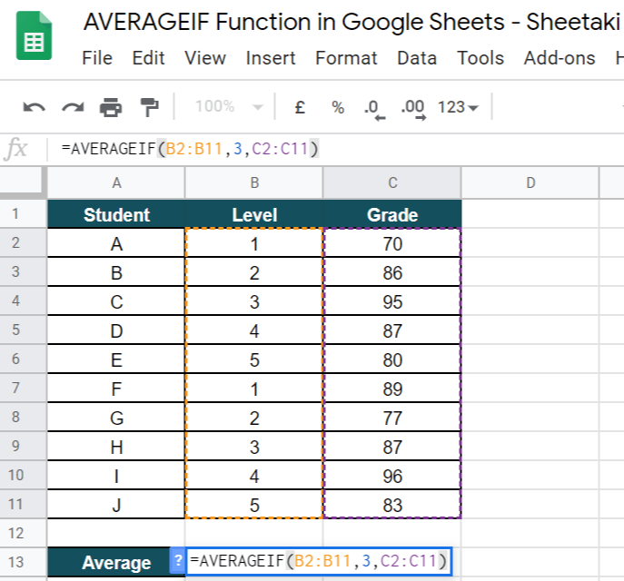
- Lastly, hit on your ‘Enter’ key. Voila! ✨

That’s pretty much it. You can now use the AVERAGEIF functions together with the other various Google Sheets formulas to create even more useful formulas that can make your life much easier. 🙂