How to Use REGEXEXTRACT Function in Google Sheets

The REGEXEXTRACT Function in Google Sheets is useful if you want to extract a certain text string within a given data.

The REGEXEXTRACT function is one of the most advanced formulas in Google Sheets. Many users try to avoid this function because of its complexity. It becomes complex if partnered with another function.

It is important to understand the REGEXEXTRACT function first, before combining it with other functions. Therefore, we created this guide.

Let’s take an easy example first.

For instance, we have a client who would like us to work on a task. He wanted us to check if there is the word “red” in the list of hair color products provided on Google Sheets.

To check this, we will use the REGEXEXTRACT function. We will add attributes such as the cells where we want to get our data from, and the text that we are trying to extract, which is, in this case, the word “red”. As easy as pie!

Let’s take another example and level it up!

Say another client of ours is selling cellphone units. He or she wants us to check if the Amazon URLs contain the brand words “Samsung”, “Apple”, and “Xiaomi”.

Using the REGEXEXTRACT function, we can easily input the range of cells where the URLs are added, and input the texts “Samsung”, “Apple”, and “Xiaomi”. Then, drag the formula down for it to work on the series of cells. Easy, right? Here’s how it looks like on Google Sheets:

As you can see in the example above, we used the REGEXEXTRACT function, added the attributes needed, then inputted the words Samsung, Apple, and Xiaomi. In the example, the formula generates the words that we are trying to extract. If it doesn’t contain the words that we asked for, it will return an #N/A value.

Additionally, the REGEXEXTRACT function is extra useful, especially when we are working on large files that are full of information. Instead of checking every cell, and spending much time in moving from one cell to another, the REGEXEXTRACT function comes in as a handy tool that helps you in those instances.

The Anatomy of the REGEXEXTRACT Function

So, the way we write the REGEXEXTRACT Function is:

=REGEXEXTRACT(text, regular_expression)

Let’s break this down to make the explanation simpler.

• = the equal sign is just how we start any function in Google Sheets.
• REGEXEXTRACT() is our function. We need to add two attributes, namely, the text and regular_expression to make it work correctly.
• text is the cell where you want to extract a certain word. In our example above, F2.
• regular_expression is the word that you want to be extracted from a given text. In our example, “Samsung”, “Apple”, and “Xiaomi”.

⚠️ Now a few notes before using the REGEXEXTRACT Function:

1. The REGEXEXTRACT function mainly and solely works for texts. If you want a numeric output, you have to pair it with a VALUE() function. If you want to input numbers, then you must convert it first using the TEXT() function.
2. The REGEXEXTRACT function may or may not be paired with other functions. It would depend on your desired output.
3. The regular_expression must be enclosed in a quote-unquote symbol “”.
4. If you want to add more than one regular_expression, you have to separate each regular_expression with a pipe or bar “|“. This connotes “or”.
5. The regular_expression may not be in an arranged manner. Meaning you can arrange in any way you like as the order does not give any precedence.

Now it may look like there’s a lot to know, especially with everything noted above. Rest assured, we will go through it and subsequently practice applying it. 🙂

A Real Example of Using REGEXEXTRACT Function

Take a closer look at the example below to see how the REGEXEXTRACT function is used in Google Sheets.

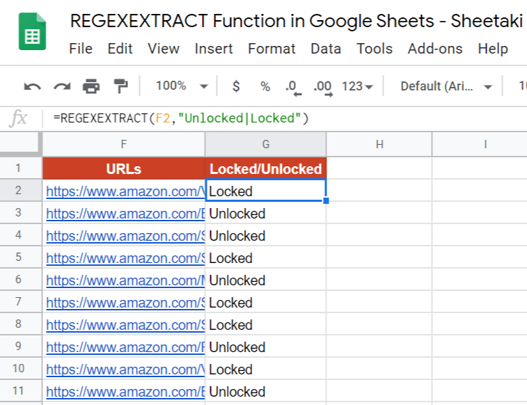
In this example, we use the REGEXEXTRACT function to determine which Amazon URLs have the words “Locked” and “Unlocked” in it.

Why have I chosen this example? Well, in a business setting, a client may want to know how many of his or her cellphone items are carrier-locked and unlocked.

To achieve this, we used this formula:

=REGEXEXTRACT(F2,"Unlocked|Locked")

Here’s what this example does:

• We selected the cell G2 because this is where we would like to write our formula.
• Secondly, we started our formula with an equal sign ‘=‘ and the function, REGEXEXTRACT.
• We opened a parenthesis and selected F2, our text. This is where our extracted output will come from.
• Fourthly, in an enclosed quote-unquote symbol, we type the regular_expression which in our case are the words “Unlocked“, followed by a pipe “|“, then another word, “Locked“.
• We closed the parenthesis and hit the Enter key to get the result.

Viola! It’s easy, right?

You may make a copy of the spreadsheet using the link I have attached below:

Have a feel on how to work with this formula. Try it out for yourself.

How to Use REGEXEXTRACT Function in Google Sheets

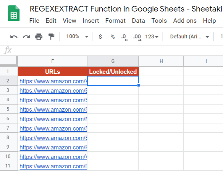
1. Simply click on any cell where you want to write down your formula. I will be choosing G2.

2. Begin your function with an equal sign ‘=‘, then followed by the name of our function, REGEXEXTRACT, then an open parenthesis ‘(‘.

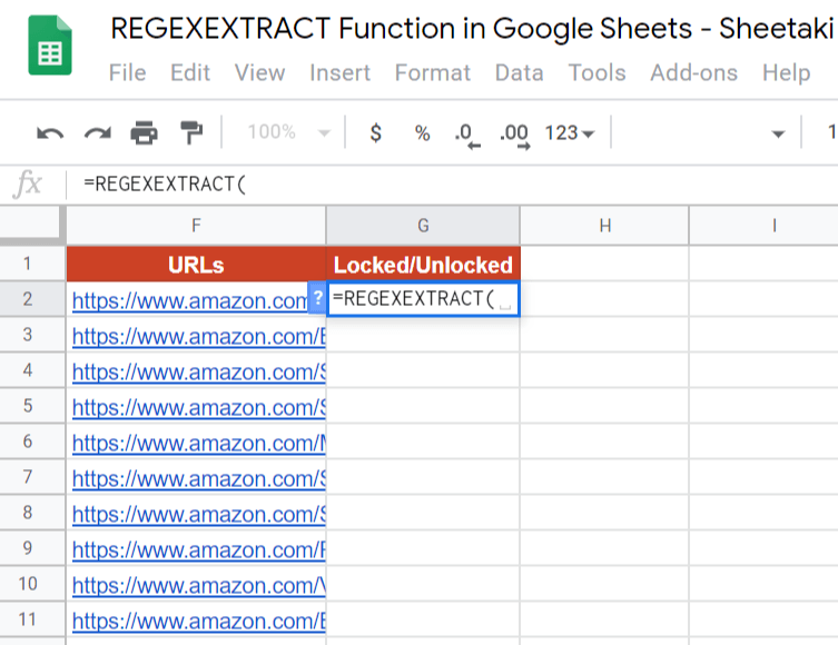
3. At this point, you should see the name of our function, REGEXEXTRACT, and an auto-suggest box where you can see an example and a summary. This will serve as your extra guide in working with the formula.

4. Column F contains the list of URLs that we are going to check. We will select the cell F2, as this is the start of the list. Furthermore, we have to add a comma ‘,‘ to separate the text from our next attribute which will be our regular_expression. Remember, our function takes two attributes: text and regular_expression.

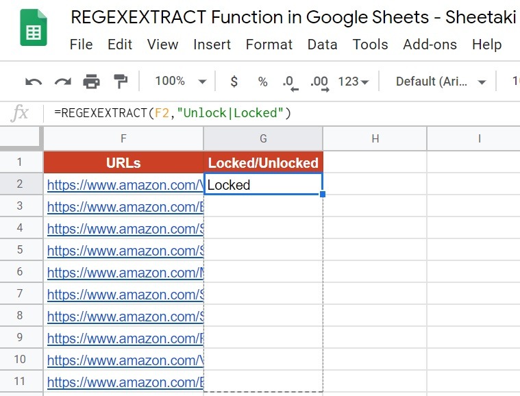
5. Next, enclosed by a quote-unquote symbol “”, type in the first regular_expression we want to look for, which is “Unlock“. Then followed by a pipe “|” since we have more than one regular_expression.

6. Still in an enclosed quote-unquote symbol, after the pipe, type the second regular_expression which we want to look for which is “Locked“.

7. Close the formula with a close parenthesis ‘)‘.

8. Finally, just hit your Enter key. Once you’ve hit the Enter key, drag the formula down to G11 by clicking on the little square on the bottom-left of the cell and dragging it down. This will apply the function on all the cells in the range from F3 to F11.

9. After following the steps above, your output should look something like this.

That’s it. Well done! 👏🏆

You can now use the REGEXEXTRACT function together with the other numerous Google Sheets formulas to create even more powerful formulas that can make your life much easier. 🙂

Get emails from us about Google Sheets.

Our goal this year is to create lots of rich, bite-sized tutorials for Google Sheets users like you. If you liked this one, you'll love what we are working on! Readers receive ✨ early access ✨ to new content.

Subscribe