How to Use the RECEIVED Function in Google Sheets

The RECEIVED function in Google Sheets is used to calculate the amount received at maturity for a specified investment in fixed-income securities purchased on a given date.

This financial function is useful because it helps you find out the future value that you will receive for an investment made on a certain date. It will be easy to calculate this with the given information.

Let’s look at an example.

You are looking to make an investment in bonds. Given a settlement date, maturity date, amount of investment, and discount rate, what is the amount you will receive at the end?

How should we go about this problem?

The RECEIVED function takes in all these inputs in order to calculate the amount received at maturity for your specified investment.

The Anatomy of the RECEIVED Function in Google Sheets

The syntax of the RECEIVED function is as follows::

=DISC(settlement, maturity, investment, discount, [day_count_convention])

Let’s look into the various sections of the function to understand how it works:

• = is the equals sign is how we start the function in Google Sheets.
• DISC is the name of our function.
• settlement is the settlement date of the security, which is the date after issuance to the buyer of the delivered security.
• maturity is the end date of the security, which is the date it can be redeemed at face value.
• investment is the amount that was invested, regardless of the actual face value.
• discount is the discount rate of the invested security.
• day_count_convention is an optional input that is an indicator of which day count method will be in use for the function. This is 0 by default.
  • 0 indicates 30/360 – the US National Association of Securities Dealers (NASD) standard of 30-day months and 360-day years.
  • 1 indicates Actual/Actual – this is the standard that is used for US Treasury Bonds, in addition to non-finance situations. It indicates the number of days between the dates and the number of days in the years between the dates.
  • 2 indicates Actual/360 – the number of days between the specified dates and 360-day years.
  • 3 indicates Actual/365 – the number of days between the specified dates and 365-day years.
  • 4 indicates 30/360 – the European standard of 30-day months and 360-day years, but adjusted in compliance with European standards of end-of-month dates

Take note that you must input the settlement and maturity dates need to be formatted, and using DATE,TO_DATE functions can help with that.

A Real Example of Using the RECEIVED Function

Let’s look at the example below to see how to use RECEIVED function in Google Sheets.

Calculating the Amount Received for a Specified Investment in Google Sheets

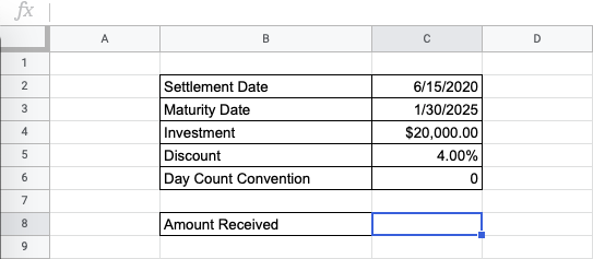
This is a simple problem. We want to find the amount to be received from a certain investment. The settlement and maturity dates are given below, and we have an investment and the discount rate. We will use the typical US standard for the day count convention.

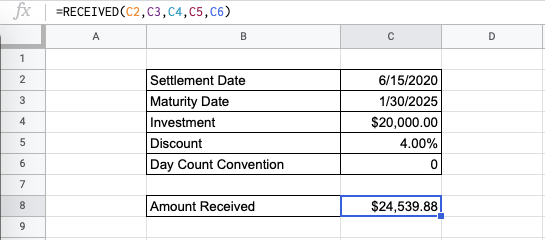
The function takes five arguments, one of which is optional. In the equation, it will look like this:

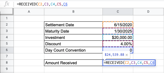
=RECEIVED(C2,C3,C4,C5,C6)

As a result, we get $24,539.88.

This simple problem can be practiced to perfection. Here’s a link so you can get a copy of this exercise:

How to Use RECEIVED Function in Google Sheets

In this section, we will show you a step-by-step process on how to use the RECIEVED function in Google Sheets.

In this problem, we will be calculating the number of interest payments it takes between the settlement and maturity date.

Calculating the Amount Received from an Investment in Google Sheets

1. Before we start, let’s make set the information of the dates provided with the DATE function. This is so we won’t encounter any errors from a mistaken input of day, month, and year.
   
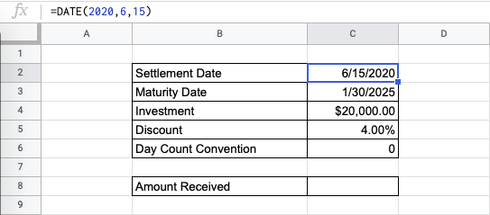
2. Then, choose a cell to make active where our desired result will show. For this guide, the answer will be in Cell C8.
   
   
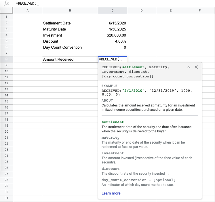
3. Next, type the equal sign ‘=’ to start. Type in “RECEIVED” or “received” – the functions that you input in Google Sheets aren’t case sensitive, so you can type in either of the above.
   
4. The auto-suggest box will create a drop-down menu. Select the RECEIVED function by clicking it.
   
   
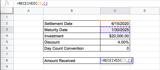
5. After the opening bracket ‘(‘, enter the settlement date attribute.
   
6. Next, we enter the maturity date.
   
7. Next, we enter the price of the investment, which what was paid on the settlement date.
   
8. Next, we enter the discount rate of the investment.
   
9. Lastly, choose the day count convention. Here we have indicated zero, but you can also leave it blank. You should be seeing the final result as a preview.
   
10. Hit enter and you’re done!
    

When solving any problems where you need to find the amount received at the end of the investment, use the RECIEVED function to find and study the correct input of dates, investment, discount rate, and conventions for your important financial decision-making.

And there you have it – you can now use the RECEIVED function in Google Sheets together with the other numerous Google Sheets formulas to create even more effective formulas.

Get emails from us about Google Sheets.

Our goal this year is to create lots of rich, bite-sized tutorials for Google Sheets users like you. If you liked this one, you'll love what we are working on! Readers receive ✨ early access ✨ to new content. There will be no spam and you can unsubscribe at any time.

Subscribe