This guide will explain how to use the FV function in Google Sheets.
Table of Contents
When we need to calculate the future value of an annuity investment based on constant-amount periodic payments and a constant interest rate, we can easily do this using the FV function in Google Sheets.
The rules for using the FV function in Google Sheets are the following:
- We need to ensure we are using consistent units for rate, number_of_periods, and payment_amount.
- By default, the present_value argument is 0.
- By default, the end_or_beginning argument is 0 meaning the payments are due at the end of each period. Otherwise, the value can be 1 if the payments are due at the beginning of each period.
Google Sheets offers several functions we can utilize to calculate different financial factors, such as the FV function.
The FV function is beneficial in financial analysis to determine the future value of our investment in a specific period of time. We consider the rate, the number of payments to be made, the payment amount, the current value, and the payment schedule.
In this guide, we will provide a step-by-step tutorial on how to use the FV function in Google Sheets. Additionally, we will explore the syntax and a real example of using the function.
Great! Let’s dive right in.
The Anatomy of the FV Function
The syntax or the way we write the FV function is as follows:
=FV(rate, number_of_periods, payment_amount, [present_value], [end_or_beginning])
- = the equal sign is how we start any function in Google Sheets.
- FV() is our
FVfunction. This function calculates the future value of an annuity investment based on constant-amount periodic payments and a constant interest rate. - rate is a required argument. This refers to the interest rate of our investment.
- number_of_periods is also a required argument. It refers to the number of payments to be made.
- payment_amount is another required argument. This refers to the amount per period to be paid.
- present_value is an optional argument. It refers to the current value of the annuity. By default, the value is 0.
- end_or_beginning is another optional argument. This refers to whether the payments are due at the end (0) or beginning (1) of each period. By default, the value is 0.
Common Mistakes in Using MIDB Function
The FV function has a straightforward syntax making it simple to use. However, we still need to be careful to ensure the function properly works.
Firstly, do not forget to convert the interest rate to a decimal. We must always divide the percentage by 100 to get the correct decimal value.
Secondly, we should ensure to use a negative value instead of a positive value. We must remember that outgoing payments should be entered as negative values.
Thirdly, ensure to specify the optional present_value and end_or_beginning arguments when needed. If we have an initial investment or need to change the payment timing, include these arguments in the formula.
Moreover, interest rate values must be added correctly. If we have a monthly interest rate and want to calculate the future value based on an annual interest rate, we can multiply the monthly rate by 12.
Additionally, make sure to use the consistent units for rate, number_of_periods, and payment_amount. For example, a house loan for 36 months may be paid monthly, in which case the annual percentage rate should be divided by 12, and the number of payments is 36.
However, a different type of loan of the same length might be paid quarterly, in which case the annual percentage rate should be divided by 4, and the number of payments would be 12.
Lastly, check the syntax of the formula. Ensure the syntax of the function call is correct, including the proper placement of commas, the use of parentheses, and quotation marks.
A Real Example of Using FV Function in Google Sheets
Let’s say we want to calculate the future value of an annuity investment based on the following data:
- an annual interest rate of 5%
- no additional payments over 10 years
- a current value of $4,000
Our initial data set would look like this:
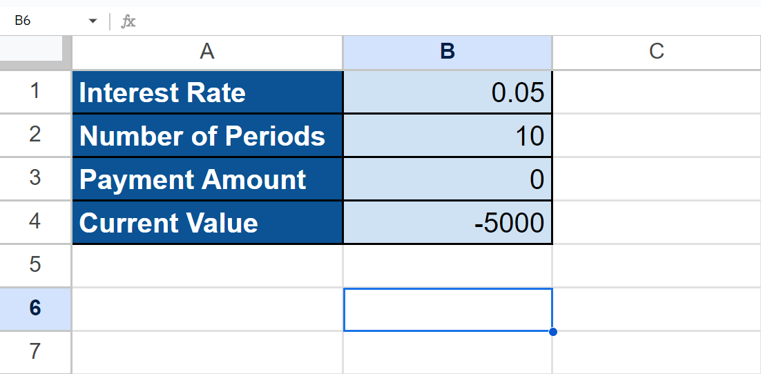
The spreadsheet above shows all the values we need to calculate the future value of the annuity investment. We have the interest rate, number of payments to be paid, payment amount, and current value.
Additionally, the current value is negative because it is an outgoing payment meaning we are releasing money and not getting money.
We can easily calculate this using the FV formula below:
=FV(B1,B2,B3,B4)
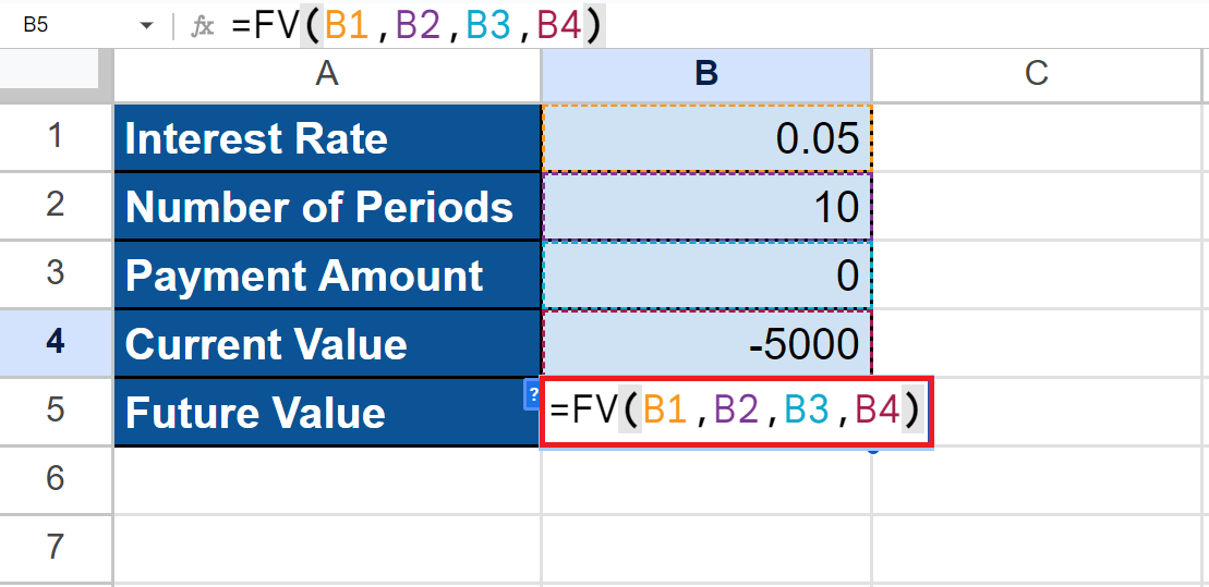
In the formula above, we first selected the cell containing the rate, which is B1 (0.05). Then, we selected the cell containing the number_of_periods, which is B2 (10).
Afterward, we selected the cell containing the payment_amount, which is B3 (0). Lastly, we selected the cell containing the present_value, which is B4 (-5000)
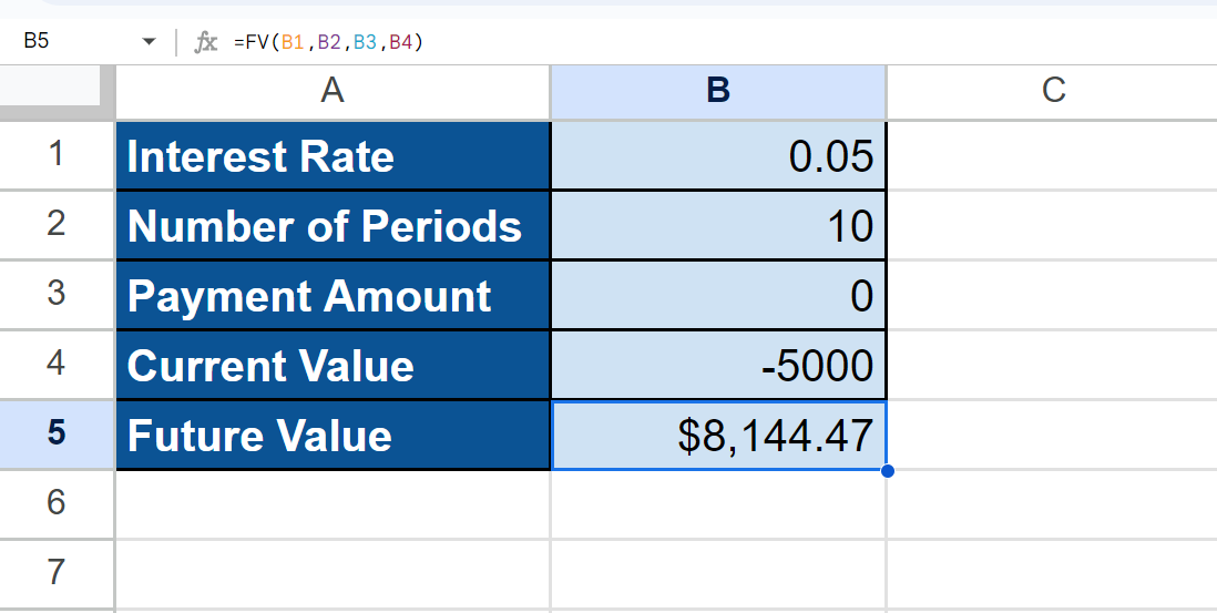
Our final data set would look like this:
You can make your own copy of the spreadsheet above using the link below.
Amazing! Now we can dive into the steps of using the FV function in Google Sheets.
How to Use FV Function in Google Sheets
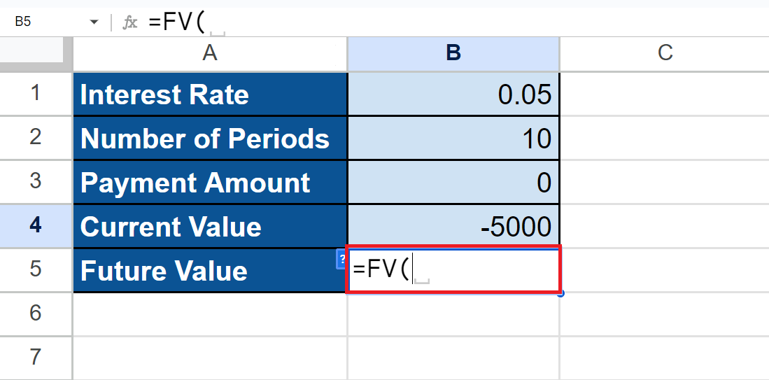
1. First, we will select an empty cell to type in our formula. To start, we will type in an equal sign and the function name. Our formula would start with “=FV(”.
2. Then, we will simply select the cells containing the interest rate, the number of payments to be made, the payment amount, and the current value of the annuity. Our final formula would become “=FV(B1,B2,B3,B4)”.

3. We will press the Enter key to return the result.

And tada! We have successfully used the FV function in Google Sheets.
You can apply this guide whenever you need to calculate the future value of an annuity investment based on constant-amount periodic payments and a constant interest rate. You can now use the FV function and the various other Google Sheets formulas available to create great worksheets that work for you.
That’s pretty much it! Make sure to subscribe to our newsletter to be the first to know about the latest guides and tutorials from us.