

IMPORTRANGE is one of the most important functions in Google Sheets. It helps the user to handle and manage multiple live spreadsheets at once effortlessly.
This means that you don’t need to manually copy and paste the data from Spreadsheet 1 to Spreadsheet 2 to keep them in sync. The IMPORTRANGE function will copy any changes made in the original spreadsheet.
Table of Contents
The rules for using the IMPORTRANGE function in Google Sheet are as follows:
- The function should have two arguments ONLY, the spreadsheet URL and the range string.
- The user must utilize the function tab in the second sheet when using the
IMPORTRANGEfunction. - To import data from the reference sheet, the user must click on the ‘Allow Access‘ prompt.
To grasp the idea of what this function is for, here is an example:
Say, for instance, you are handling a set of students who volunteered to make a sustainable future. Your task is to keep track and update the student’s data in several spreadsheets specifically intended for different departments.
Instead of manually inputting every student’s information to the second independent sheet, you can use the IMPORTRANGE function to import the students’ data automatically.
Are you wondering how to do it?
Let me tell you more about the IMPORTRANGE Function. Let us start with the correct way to write it.
The Anatomy of the IMPORTRANGE Function
So the syntax (the way we write) the IMPORTRANGE function is as follows:
=IMPORTRANGE(SpreadsheetURL,RangeString)
Let’s cut it up and learn the essential parts of the function.
- = every function in the google sheet always starts with an equal sign. This is used to notify the spreadsheet that you are working on a formula and not plain text.
- IMPORTRANGE is a Google Sheet function that will help you automatically import and sync live data from one spreadsheet to another.
- Spreadsheet URL or Spreadsheet Key refers to the source sheet where you will copy the data.
- Range String refers to the cells, columns, or rows you want to copy from the main spreadsheet.
A Real Example of Using IMPORTRANGE Function
Here’s an example of the IMPORTRANGE function used in a Google Sheet spreadsheet.
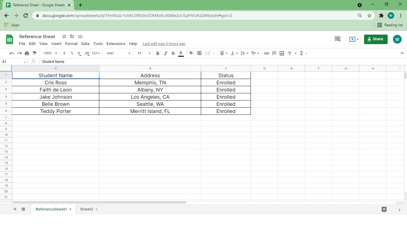
1. The first image shows the source sheet of the data that we need to copy to the second sheet.
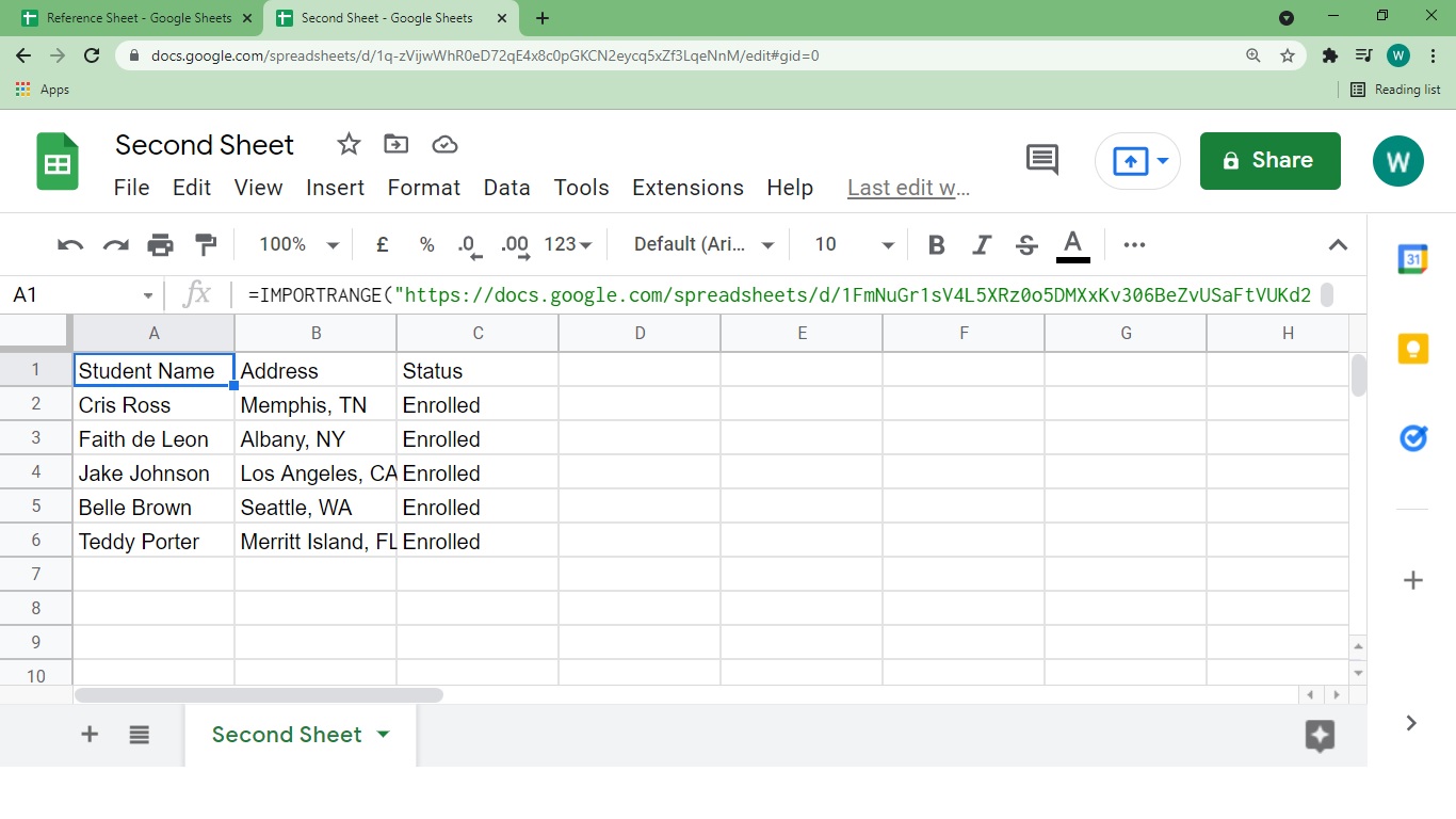
2. Here’s a screenshot of the data imported from Sheet1:
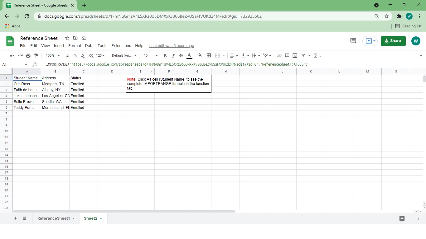
By following the correct format of the ImportRange formula, you can effortlessly copy the entire data to another sheet.
Did you notice how I wrote the IMPORTRANGE function?
To further understand how it was done, I will walk you through how to use IMPORTRANGE in Google Sheets.
You may click on the link below to copy the spreadsheet that we will be using as we proceed.
Let us now practice using the ImportRange Function.
How to Use ImportRange in Google Sheets
1. Prepare the source sheet from where you will import the data. Here’s a sample of a reference sheet.
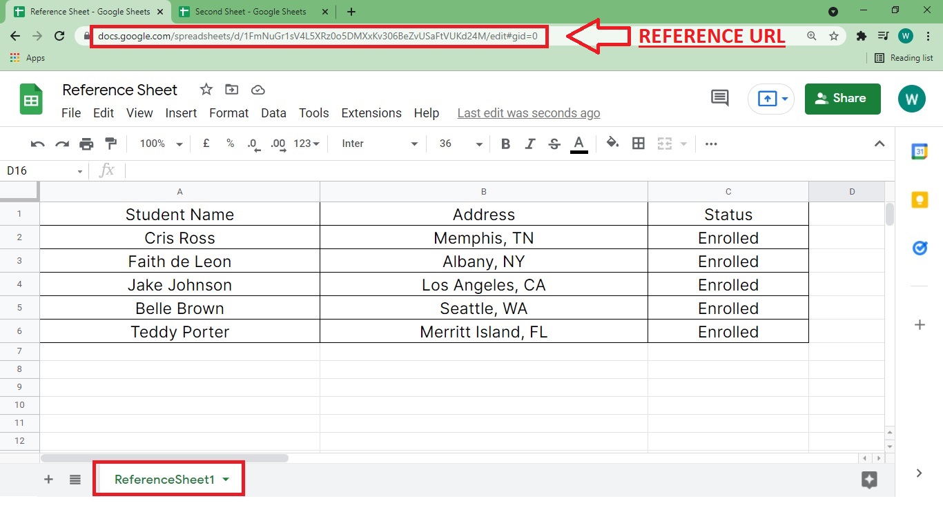
 2. Copy the source sheet’s URL or the spreadsheet key.
 3. Open the second sheet, and locate the function tab. The second sheet could either be inside the same spreadsheet or a separate sheet. Both should be able to import data.
In this example, I use a completely separate spreadsheet.
 4. Input the
 IMPORTRANGE formula in the function tab of the new spreadsheet. Start it with the equal sign ‘=‘ before putting the IMPORTRANGE function. It should look like this:

5. Then, add an open parenthesis ‘(‘ followed by a quote sign ‘“‘.

6. Once done, paste the reference URL or the spreadsheet key followed by a quote sign ‘“‘.
In this step, the function’s syntax should look like this:

Now that we are done adding the source’s URL, we will add the string range.
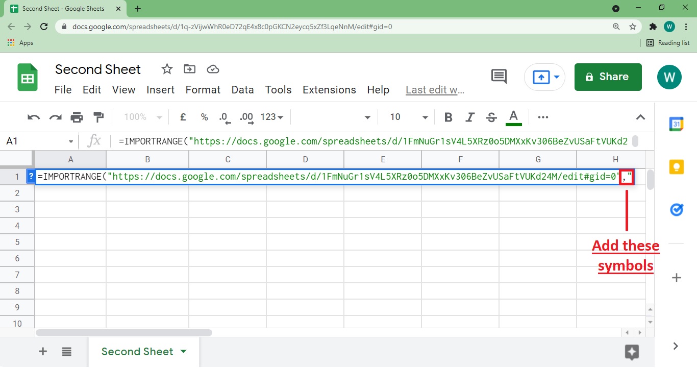
7. Right after the quote symbol ‘“‘, add a comma ‘,‘ followed by a quote sign ‘“‘.
 8. Add the range string that you want to copy. It should look like this, ReferenceSheet1!A1:C6. This means that we will be importing the data from a sheet named ‘ReferenceSheet1 that covers cells A1 to C6.
 9. Add a quote sign ‘“‘ again followed by a closing parenthesis ‘)‘ and hit enter.
The whole IMPORTRANGE function should now look like this:
 10. Once you perform the function successfully, you will see a ‘#REF!’ message in the new sheet. Click it.
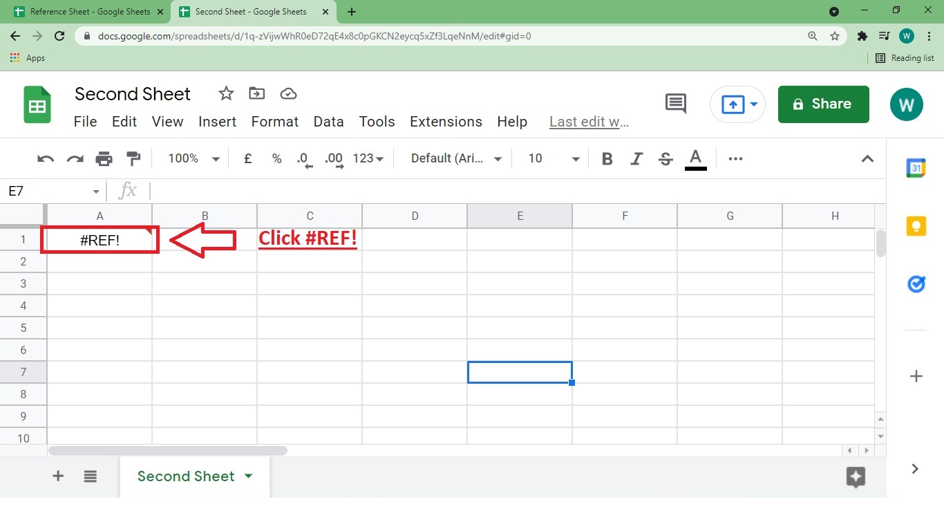 11. After clicking it, the Allow Access message will pop up. You just need to click Allow Access to import data from the source sheet to the destination sheet.
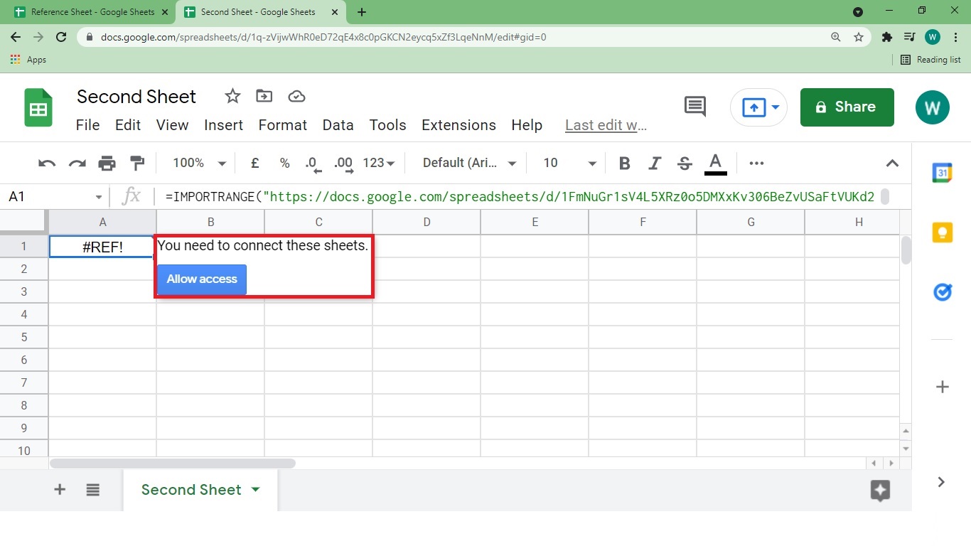 12. After clicking on Allow Access, here’s what you will see next.
Take note: What will be imported is just the data. The font size, borders, and other elements will not or might not be copied. The imported data will use the default settings of the new spreadsheet.
Frequently Asked Questions (FAQ)
Yes.
1. Will IMPORTRANGE function in the same spreadsheet?
Yes. The formula will work on the same spreadsheet. As long as you write the formula correctly, the second sheet can import the data successfully.
2. Can you use IMPORTRANGE without putting the cell’s column number and row number?
Yes. But instead of writing A1:B:100 as a range string, you need to input A:B.
Were you able to follow through? Do you still need more practice? If so, keep the link that we used and keep practicing. Feel free to play around with the link until you master the IMPORTRANGE Function. Once you do, let us know by dropping a comment below.
Don’t forget to sign up for our newsletter for you not to miss any informational articles like this. Also, you may check on the article below if you want to pull exact data from your google spreadsheet through IMPORTRANGE.


