The TRIMMEAN function in Google Sheets is used to calculate the mean of a dataset excluding some proportion of data from the high and low ends of the dataset.
Table of Contents
This function is useful because it helps you to find and remove the outliers in a given data set and return the mean or average.
The function’s parameters on the proportion of the dataset outliers can be specified by the user. TRIMMEAN will exclude these data points in the calculation and return the adjusted mean or average accordingly.
Let’s look at an example.
You have a spreadsheet that details your exercise plan on your high-intensity interval training. You want to know your average number of reps you have in each exercise. However, you notice that you have some days where you did extraordinarily well and other days where you did not. You want to get a good picture of your average reps.
How should we go about this problem?
The TRIMMEAN function make a more insightful calculation for the average of a data set. It is a helpful tool that will allow for such a calculation to take place in a neat manner.
The Anatomy of TRIMMEAN Function in Google Sheets
The syntax of the TRIMMEAN function is as follows:
=TRIMMEAN(data, exclude_proportion)
Let’s have a look at each part of the function to understand what is going on here:
=is the equals sign that starts off any function in Google Sheets.TRIMMEANis the name of our function.datais the array or range containing the dataset to consider.exclude_proportionis the proportion of the dataset to exclude, from the extremities of the set. This must be a percent that greater than or equal to zero or less than 1.
This way the TRIMMEAN function works is that it will first remove the outliers as the user indicated in the formula. Then, it will calculate the average over the new data set.
A Real Example of Using TRIMMEAN Function
You may be curious as to why the TRIMMEAN function exists, when there are other ways to calculate averages.
The TRIMMEAN function helps to remove outliers that may skew the data and affect any of your conclusions. This is helpful in a variety of very specific tasks.
Let’s look at the example below to see how to use the TRIMMEAN function in Google Sheets.
Calculating the average of array values in Google Sheets
This is a simple problem. It is a simplified task to help you understand what the function can be used for.

In the equation, it will look like this:
=TRIMMEAN(C3:C12,0.2)
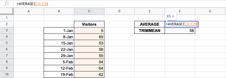
It will result in an average of 56.
While the regular AVERAGE calculates it as 72, you will notice a couple of instances that are vastly different from the other days. The TRIMMEAN takes note of this and calculates the average without these outliers.
This is how the function works in this example: There are 10 data points in the example. The percentage that was indicated was 0.2 or 20%. 20% of 10 data points is 2. What then happens is that the 1 highest data point and 1 lowest data point will be removed from the data set.
This simple problem can be practiced to perfection. Use the link below to get a copy of this problem set:
How to Use TRIMMEAN Function in Google Sheets
In this section, we will show you a step-by-step process on how to use the TRIMMEAN function in Google Sheets.
In this problem, we will find the average.
Using TRIMMEAN Function In Google Sheets
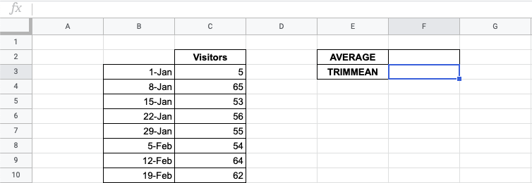
- To begin, prepare your spreadsheet with the information you want to check.

- Start to fill in the
TRIMMEANfunction. In this example, we pick cell F3.
- Start by adding in the TRIMMEAN function.
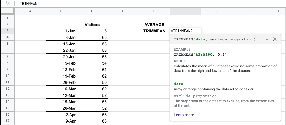
- Start by putting in the array of data you want to analyze.

- Next, input the exclude_proportion value. We choose 20% in the example. You can input it as 20% or 0.2. Note that you’ll get a preview.

- Next, hit enter. You are done!
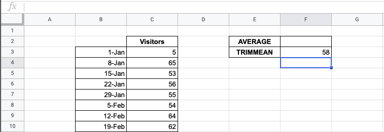
- Compare this to the average. You’ll notice that they are significantly different values.
The TRIMMEAN function can help make accurate findings from your data.
And there you have it – you can now use the TRIMMEAN function in Google Sheets together with the other numerous Google Sheets formulas to create even more effective formulas.