How to Use DCOUNTA Function in Google Sheets

This guide will explain how to use the DCOUNTA function in Google Sheets.

The DCOUNTA function is a powerful built-in Google Sheets function that allows you to count the number of cells within a specified range that follows specific criteria. 

This function is useful when working with larger datasets or when you need to consider two or more criteria. 

For example, you may want to know the number of non-empty cells that have a value less than $1000 in the ‘Price’ column and a rating greater than 3.5 in the ‘Rating’ column.

In this guide, we will provide a step-by-step tutorial on how to use the DCOUNTA function in Google Sheets. Additionally, we will cover how to format your complex criteria into an array that can be referenced in the DCOUNTA function.

The Anatomy of the DCOUNTA Function

The syntax of the DCOUNTA function is as follows:

=DCOUNTA(database, field, criteria)

Let’s look at each argument to understand how to use the DCOUNTA function.

• the database argument refers to the array or range containing the data you want to use as a database. The data must have an initial header row that contains labels for each column.
• the field argument indicates which column in the database argument you want to operate on. 
• the criteria argument will be an array or range containing zero or more criteria to filter the database values by.
• If you only need to count the number of non-blank cells in a range, we recommend using the COUNTA function instead.

A Real Example of the DCOUNTA Function

Using the DCOUNTA Function with a Single Criteria

Let’s explore a simple example where we’ll use the DCOUNTA function to count values in a dataset.

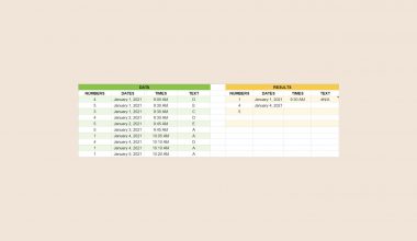
In the table above, we have a dataset of products. Each row contains the product ID, category, product price, and number of reviews. We want to count the number of products that have less than ten reviews.

In the example above, we used the following formula to find the number of products with less than 10 reviews:

=DCOUNTA(A1:D13,"Product ID",{"Reviews";"<10"})

The DCOUNTA function reveals that only 7 of our products have less than 10 reviews. Do note that the criteria in the third argument must be an array where the first row is a valid field and the second row is the actual criteria to use.

Since we only have one criteria, we can write our third argument using the array syntax {“Field”;”criteria”}. 

Using the DCOUNTA Function with Array of Criteria

Let’s take a look at a second example where we’ll use DCOUNTA to count values using two or more criteria.

In the example above, we have an array of criteria in the range F2:H3. We want to find the number of products that match the following criteria:

• Less than twenty reviews
• A price greater than $500
• In Category B

We’ll use the following formula to find the number of products that fit our criteria:

=DCOUNTA(A1:D13,A1,F2:H3)

Instead of including our criteria manually in the formula, we’ll refer to our criteria range F2:H3. We’ll also refer to the field to count (‘Product ID’) using a cell reference instead (A1). 

Google Sheets also supports using multiple rows for the criteria array.

In the table above, our criteria range has expanded to two rows. The two rows define the following criteria for our DCOUNTA function:

• the product is from category B, has over 20 reviews, and has a price less than $500
• or the product is from category A

In Google Sheets, each expression within the same criteria row is joined with AND logic. Each criteria row is then joined with OR logic.

In the example above, we’ll use the updated criteria array with our DCOUNTA function:

=DCOUNTA(A1:D13,A1,F2:H4)

Our DCOUNTA formula reveals that five products match our criteria. The two rows in our dataset highlighted in blue are included because they follow the criteria in the first row. The three rows highlighted in yellow are included because of the criteria defined in the second row.

Click on the link below to create your own copy of our examples.

Head to the next section to read our step-by-step tutorial on using the DCOUNTA function in Google Sheets.

How to Use the DCOUNTA Function in Google Sheets

1. Select the cell where you want to place the DCOUNTA function.
   
2. Type the DCOUNTA function and enter the range you wish to use as a database.
   In the formula above, we’ll use the range A1:D13 as our database.
   
3. Enter the name of the column you want DCOUNTA to count. Ensure that the value matches the actual header value from the selected database.
   
4. Enter an array with your desired columns and criteria. The first value must be the name of a valid column in your database. The second value must be a valid criteria string.
   Hit the Enter key to evaluate the DCOUNTA function.
   
5. When working with multiple criteria, arrange them into a 2-row array in your spreadsheet.
   
6. Type the cell reference to your sheet’s criteria array as the third argument of your DCOUNTA function.
   

These are all the steps you need to follow to start using the DCOUNTA function in Google Sheets.

FAQs

1. What is the difference between DCOUNT and DCOUNTA?
   The DCOUNT function strictly counts numerical values only, while the DCOUNTA function counts all non-blank cells (both numeric and text values).

To learn more about counting values based on criteria, you can read our post on how to use the SUBTOTAL function with COUNTIF.

That’s all for this guide! Be sure to check out our library of spreadsheet resources, tips, and tricks!