How to Use the AGGREGATE Function in Excel

This guide will explain how to use the AGGREGATE function in Excel.

Aggregate functions are an important tool for data analysis. Functions such as COUNT, AVERAGE, and SUM allow you to summarize your data and create reports. 

Excel’s AGGREGATE function can be used to analyse a dataset by applying a specified aggregate function. The function is also useful because it can be set to ignore hidden rows, nested subtotals, and cells with errors.

In this guide, we will provide a step-by-step tutorial on how to use the AGGREGATE function to apply different aggregate functions to a list or database.

The Anatomy of the AGGREGATE Function

The syntax of the AGGREGATE function is as follows:

=AGGREGATE(function_num, options, ref1, [ref2], …)

Let’s look at each argument to understand how to use the AGGREGATE function.

• = the equal sign is how we start any function in Excel.
• AGGREGATE() refers to the AGGREGATE function. The function allows us to return an aggregate of a list or database with the ability to ignore hidden rows and error values.
• function_num controls the aggregate function to use. This argument must be an integer from 1 to 19. For example, a function_num of 1 will set the aggregation function to AVERAGE.
• The options argument is a numerical value that determines which values to ignore in the provided range.
• The ref1 number must be the first numeric argument that you want to aggregate.
• ref2,… refers to the remaining numerical arguments you wish to aggregate.
• For certain aggregate functions (such as LARGE and SMALL), the second argument is required since the function needs both an array and another parameter.

A Real Example of Using the AGGREGATE Function in Excel

AGGREGATE Function Numbers

Before diving into the AGGREGATE function, let’s take a look at each of the available aggregate functions you can use and their respective function number or code.

Aggregate Function Options

After selecting the aggregate function to use, we’ll need to provide another number for the options argument. 

Here are the possible choices and their respective behavior:

• If no options are provided (or if set to 0), AGGREGATE will ignore the nested SUBTOTAL and AGGREGATE functions.
• A value of 1 will make AGGREGATE ignore hidden rows (along with nested functions)
• A value of 2 will make AGGREGATE ignore error values (along with nested functions)
• A value of 3 will make the function ignore hidden rows, error values, and nested SUBTOTAL and AGGREGATE functions.
• Inputting a value of 4 will ensure that the AGGREGATE function does not ignore any rows when aggregating.
• A value of 5 will ensure that the country ignores just hidden rows
• A value of 6 will ensure that the function ignores just cells with error values
• A value of 7 will indicate that we want to ignore all hidden rows and error values.

Now that we know the functions and options available, let’s look into a few simple examples where we can use the AGGREGATE function.

Using AGGREGATE To Find the SUM of a Range

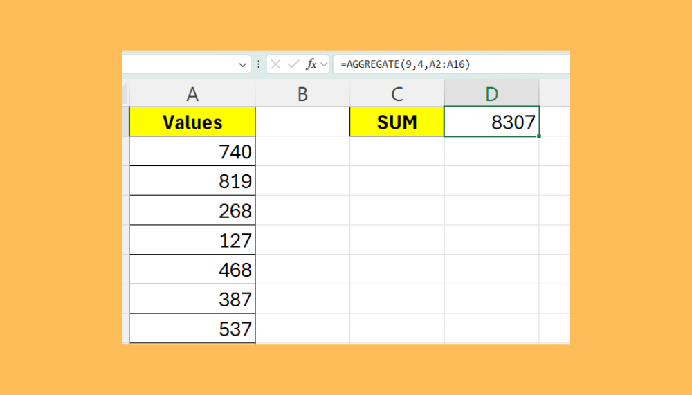
Let’s try using the AGGREGATE function to find the sum of a range.

In the table above, we have a list of values we wish to find the sum of. We can use the following AGGREGATE formula to determine the total sum:

=AGGREGATE(9,0,A2:A16)

In the formula above, we provided a function code of 9 to indicate we want to use the SUM aggregate function. We’ll set the options argument to the default value of 0. The last argument indicates the range we wish to aggregate.

After evaluating the AGGREGATE function, our cell should now display the total of the selected range.

Another useful feature of the AGGREGATE function is the ability to ignore filtered or hidden rows.

In the example above, we used the AGGREGATE function to find the average sales from a filtered dataset that contains a breakdown of sales by city. The current spreadsheet has the range filtered to only show two cities.

If we adjust the filter to show all cities, our AGGREGATE function will automatically update. To achieve this behavior, the options argument must be set to an option that ignores hidden rows.

Click on the link below to create your own copy of our examples.

Head to the next section to read our step-by-step tutorial on how to use the AGGREGATE function in Excel.

How to Use the AGGREGATE Function in Excel

1. You must first identify the range in your spreadsheet that you wish to aggregate and which aggregate function to use on that range. Next, identify the cell where you wish to output the result of the AGGREGATE function
   
   In this example, we’ll aggregate the range A2:A16 by using the SUM function. We want to output the result in cell D1.
   
2. Select the target cell and type “=AGGREGATE(“ to start the AGGREGATE function. As the first argument, enter the function code associated with your desired aggregate function.
   
   Next, enter your desired behavior for the options argument. For this example, we’ll select the “Ignore nothing” behavior by typing in 4.
   
   Lastly, enter the range of cells you wish to aggregate.
   
   In this example, we’ll select the cell range A2:A16 to aggregate.
   
3. Hit the Enter key to evaluate the function.
   
   In our example above, we’ve determined that the sum of the range A2:A16 is 8,307.

To learn more about using Excel to aggregate data, you can read our post on how to sum filtered rows in Excel.

That’s all for this guide! Be sure to check out our library of spreadsheet resources, tips, and tricks!