Learning how to apply conditional formatting based on another cell in Google Sheets is useful to analyze a large amount of data across the sheet based on a set of conditions.
It is common to apply conditional formatting based on the current value to help visualize or emphasize an unusual value. However, we can also apply conditional formatting based on another cell’s value by inputting certain custom conditions.
Something to take note of is that color scale can only be applied to numbers, including date and time. If the cell contains numbers together with text, it would not use the color scale feature in Google Sheets.
However, do not fear as you can always extract the numbers into another cell by using the REGEXTRACT or REGEXREPLACE functions. You can then apply a color scale to the new cells.
Table of Contents
Let’s take an example:
Imagine you run a business, and would like to analyze the performance of your products. You sell various kinds of products, and it is time-consuming to look through them one by one to identify them.
Hence, by using the conditional formatting based on another cell in Google Sheet, you would minimize the time used to analyze this data. Applying conditional formatting helps you look at all the problem areas in one glance.
For example, here are the products you sell. You would like to see which products are not performing well.
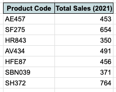
You then set a benchmark signifying that any product selling more than $400 is considered healthy. Otherwise, the product that did not hit the $400 mark would need to be reevaluated.
By applying the conditional formatting on the product code based on the total sales achieved in the year 2021, the product codes that did not reach the benchmark would be highlighted in red.

As we can see, product code with HR843 and SBN039 failed to meet the benchmark and needs reevaluation if sales would be continued.
A Real Life Example of Applying Conditional Formatting Based on Another Cell in Google Sheets
In this example, picture yourself as a bakery owner. You keep a stock sheet and record all movements when ingredients are used and purchased.
Every month, you would need to take note of which items are low in stock. This is done to make sure the items are repurchased, and there are enough ingredients for baking in the coming month.
To quicken the process, we can apply conditional formatting on all ingredients based on the amount of stock left at month-end.
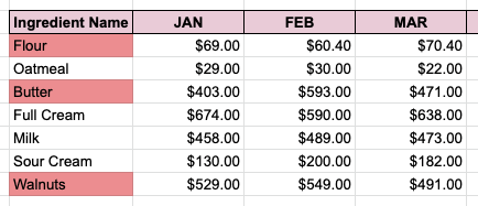
We will then set a benchmark that signifies the stock is low. Let’s say ten units of an ingredient left is considered as low in stock. Any stock with 10 units or less than would be colored in Red.

As you can see, it is clear that you would need to purchase full cream, milk, and sour cream soon!
You may make a copy of the spreadsheet using the link I have attached below.
How to Apply Conditional Formatting Based on Another Cell in Google Sheets
Example 1
- First, we select the range we want to apply the conditional formatting. In this example, it would be B3:B9.

- Then, you select Format, then click Conditional formatting.

- Once you clicked Conditional formatting, a Conditional format rules pop-up on the side would appear.

- We will need to click the dropdown box for the format rule and choose Custom Formula to create our own formula.

- As we would like to apply color to the ingredient with less than ten units left, we would key in ‘=C3<=10‘.

- We would then choose the color Red to express a sense of urgency. Once all the above are completed, you can click Done.

- When you press Done, your sheet will look like this.

Example 2
Conditional formatting based on another cell is not limited to only one cell. You can apply conditional formatting on several other cells altogether in Google Sheets.
In another scenario, you noticed that this year’s profit margin is much lower compared to previous years. After a general inspection, you realized that this is due to the increased cost of baking this year.
The amount of data you need to go through for all the costs incurred the whole year looks like a nightmare! 😫
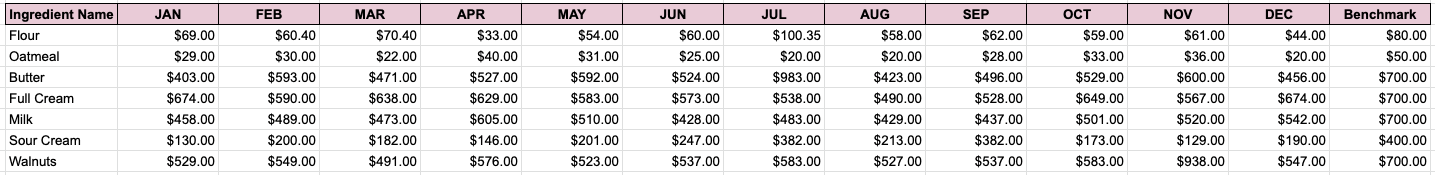
By applying the conditional formatting on the ingredient names based on the cost of ingredients for all months, we can then help identify which month the cost is unexpectedly high.
We then set a benchmark that is relevant to the type of ingredient.
Once the formatting is applied, you can see that if the costs for each ingredient of a certain month have exceeded the benchmark will be highlighted in Red.

To further investigate, we can then apply the conditional formatting on each month to highlight specifically which month the cost surpassed the benchmark.

- First, we select the range that we want to apply the conditional formatting on. In this example, it would be B3:B9.

- Similar to the steps explained for Example 1, you select Format, then click Conditional formatting, then choose Custom Formula to create our own formula.
- As in this example, we are depending the conditional formatting on more than one cell, the formula would look like this, =OR(C3>O3,D3>O3,E3>O3,F3>O3,G3>O3,H3>O3,I3>O3,J3>O3,K3>O3,L3>O3,M3>O3,N3>O3)
- Once you press done, your sheet will look like this.
- The highlighted ingredient names are those with months that exceeded the benchmark given.
- To gain a clearer picture on which months exceeded the benchmark for the specific ingredient, we can also apply conditional formatting on each of the months.
- To do so, we will select the cells for the highlighted ingredient. In this case, it will be C3:N3.

- Instead of choosing Custom formula, we will select Greater Than. Then, input the benchmark given.

- Once you press Done, the specific cell that exceeded the given benchmark will be highlighted.

- Repeat the same steps for Butter and Walnuts, and your sheet will look like this.
By identifying the specific months and ingredients that exceeded the benchmark, you can now explore the reason for the unexpected increase in cost in that specific month.
There you go! As shown in the examples, the conditional formatting function based on other cells can help you visualize and organize massive amounts of data.
If you are not familiar with the conditional formatting feature on Google Sheets, go ahead and check out our tutorial on how to apply it.
Don’t be afraid to try out different format rules and customizations to tailor the conditional formatting to your preferences!