This guide will discuss how to calculate autocorrelation in Excel using two easy and simple methods.
Excel is an excellent tool to use for different situations. Since it has several built-in functions and tools, we can easily perform complex and long calculations. For instance, we want to easily calculate a data set’s autocorrelation.
So autocorrelation is a type of correlation that is used to measure the degree of similarity between a time series and a lagged version of the time series over successive time intervals.
Furthermore, autocorrelation is also called serial correlation or lagged correlation because it measures the relationship between the current values of a variable and the past values. Additionally, we can use autocorrelation to easily predict future values by referring to the past values of the data set.
However, there is no single function in Excel to automatically calculates autocorrelation. But, we can utilize the different built-in functions in Excel to create a single formula that would calculate the autocorrelation.
In this guide, we will discuss two methods to calculate autocorrelation using a combination of the different built-in functions in Excel.
Let’s take a sample scenario wherein we need to calculate autocorrelation in Excel.
Suppose we have data set containing the total number of sales during 10 different time periods. And you want to calculate the autocorrelation of the data set.
Since there is no built-in function in Excel to do this, you create a single formula using the SUMPRODUCT, OFFSET, AVERAGE, and DEVSQ functions to calculate autocorrelation.
Before we move on to a real example of calculating autocorrelation in Excel, let’s first learn the syntax of the functions we will be using.
The Anatomy of the DEVSQ Function
The syntax or the way we write the DEVSQ function is as follows:
=DEVSQ(number1, [number2])
Let’s take apart this formula and understand what each term means:
- = the equal sign is how we activate any function in Excel.
- DEVSQ() refers to our
DEVSQfunction. And this function is used to return the sum of squares of deviation of the data points from their sample mean. - number1 is a required argument. So this refers to 1 to 255 arguments, array, or an array cell references, which we want the
DEVSQto calculate. - number2 is another required argument. And this serves as an additional argument that we also want the
DEVSQto calculate.
The Anatomy of the VAR.P Function
The syntax or the way we write the VAR.P function is as follows:
=VAR.P(number1, [number2])
Let’s take apart this formula and understand what each term means:
- = the equal sign is how we begin any function in Excel.
- VAR.P() is our
VAR.Pfunction. And this function is used to calculate the variance based on the entire population. Additionally, this function will ignore the logical values and text in the selected population. - number1 is a required argument. So it refers to 1 to 255 numeric arguments corresponding to a population.
- number2 is an optional argument. And this is used as additional arguments that we also want to include to calculate the variance of a population.
Great! Now we can dive into a real example of calculating the autocorrelation in Excel.
A Real Example of Calculating Autocorrelation in Excel
Let’s say we have a data set containing the total number of sales of a certain product during 10 different time periods. And we want to calculate the autocorrelation of this data set. So our initial data set would look like this:

Since Excel does not have a built-in function that will automatically calculate autocorrelation, we need to create a single formula using other built-in functions to get the autocorrelation. And there are two methods we can do this.
Firstly, we can utilize the SUMPRODUCT, OFFSET, AVERAGE, and SEVSQ functions to calculate autocorrelation in Excel. For example, we want to get the autocorrelation of the total sales for a range of lags between 1 to 4.
To do this, we will first calculate the total number of months for determining the series using the COUNTA function. Then, we will apply our formula to get the autocorrelations between the lags 1 to 4. So the OFFSET function will extract the range with the height of the rows based on the inputted reference.
Next, we will get the average value of this specific range. Afterward, the DEVSQ function will return the sum of the squares of the deviations of the range from their mean.
Secondly, we can use a formula combining the SUMPRODUCT, AVERAGE, and VAR.P functions to get the autocorrelation. Similarly, we will use the COUNTA function to determine the total number of rows in the data set.
Next, we can apply our formula to get the autocorrelations for the product between the lags 1-4. So the AVERAGE function will return the average value of the selected range. Then, the formula will find the variance based on the entire range.
Lastly, the function will return the autocorrelation for the specific lag. To calculate the next lag, we simply have to change the range we input in the formula depending on the number of lags.
So our final data set would look like this:

You can make your own copy of the spreadsheet above using the link attached below.
Amazing! Now we can move on and explain the steps of how to calculate autocorrelation in Excel.
How to Calculate Autocorrelation in Excel
In this section, we will explain the step-by-step process of how to calculate autocorrelation in Excel using two simple methods. Furthermore, each step contains detailed instructions and pictures to guide you along the way.
1. Firstly, let’s try our first method using a formula combining the SUMPRODUCT, OFFSET, AVERAGE, and DEVSQ functions. So we will first determine the number of months for the time series. To do this, we will input the formula “=COUNTA(B2:B11)”.

2. Secondly, we will now determine the autocorrelations between the lags 1 to 4. And we need to first create a new table to input the lags and results.
Then, we can type in the formula “=SUMPRODUCT(OFFSET($C$2:$C$11,0,0,$C$12-E2)-AVERAGE($C$2:$C$11),OFFSET($C$2:$C$11,E2,0,$C$12-E2)-AVERAGE($C$2:$C$11))/DEVSQ($C$2:$C$11)” for lag 1.

3. Thirdly, we will drag the Fill Handle tool down to copy and apply the formula to the other lags.

4. And tada! We have successfully calculated autocorrelations using the first method.

5. Next, let’s try our second method using the SUMPRODUCT, AVERAGE, and VAR.P functions. Similarly, we will first get the number of months in our data series. To do this, we will input the formula “=COUNTA(B2:B11)”.

6. Then, we will create a new table to input the number of lags and results. Afterward, we will type in the formula “=(SUMPRODUCT(C2:C10-AVERAGE(C2:C11),C3:C11-AVERAGE(C2:C11))/C12/VAR.P(C2:C11))”.
To get the autocorrelation of the other lag, we simply need to change the inputted range. For instance, we will exclude the first two and last two values in the data set for lag 2. Furthermore, we will exclude the first three and last three values in the data set for lag 3.

7. And tada! We have calculated autocorrections in Excel.
And that’s pretty much it! We have explained how to calculate autocorrelation in Excel using two simple and easy methods. Now you can choose any method and apply it to your work.
Are you interested in learning more about what Excel can do? You can now use the DEVSQ function and the various other Microsoft Excel formulas available to create great worksheets that work for you. Make sure to subscribe to our newsletter to be the first to know about the latest guides and tutorials from us.