


This guide will discuss how to calculate the root mean square error in Excel using three simple and easy methods.
Table of Contents
Since it has several built-in functions and tools, Excel makes it easy for us to perform complex and long statistical calculations. For instance, we can easily do regression analysis in Excel, a technique that helps us understand the relationship between two variables or data sets.
Specifically, we will focus on calculating the root mean square error in Excel. So the root mean square error or also known as the RMSE, is used to measure how much error there is between two data sets.
Basically, the root mean square error compares the forecasted values and the actual or known values. When we calculate the root mean square error for our data set, we can determine how far apart or near our forecasted values are from our actual values on average.
Furthermore, the smaller the root mean square error for our data set, the closer the forecasted values and the actual values are. Moreover, we can utilize the RMSE formula to calculate the root mean square error of any model that produces forecasted values which will be compared to the actual values.
To calculate the root mean square error in Excel, we will utilize the different built-in functions, such as the SUMSQ function, the AVERAGE function, the COUNTA function, and the SQRT function.
Let’s take a sample scenario wherein we need to calculate the root mean square error in Excel.
Suppose you have a data set containing a column for forecasted values and another for actual values. And you want to understand the relationship between the forecasted and actual values by measuring how far apart the two values are from each other.
To do this, you decided to calculate the root mean square error of your data set by using a formula that combines the SUMSQ function, the COUNTA function, and the SQRT function.
Before we learn the three simple and easy methods of how to calculate the root mean square error in Excel, let’s first understand the syntax of the functions we will be using.
The Anatomy of the SUMSQ Function
The syntax or the way we write the SUMSQ function is as follows:
=SUMSQ(number1, [number2])
Let’s take apart this formula and understand what each term means:
- = the equal sign is how we activate any function in Excel.
- SUMSQ() is our
SUMSQfunction. And this function is used to return the sum of the squares of the selected arguments. We can also input numbers, arrays, names, or cell references containing numbers as arguments. - number1 is a required argument. So this refers to 1 to 255 numbers, names, arrays, or cell references to arrays in which we want to get the sum of the squares.
- number2 is an optional argument. And this serves as an additional argument in which we also want to get the sum of the squares.
The Anatomy of the SQRT Function
The syntax or the way we write the SQRT function is as follows:
=SQRT(number
Let’s take apart this formula and understand what each term means:
- = the equal sign is how we begin any function in Excel.
- SQRT() refers to our
SQRTfunction. And this function is used to return the square root of the selected number. - number is the only argument needed for this function. So this refers to the number we want to get the square root.
Great! Now we can move on and dive into three simple ways how to calculate the root mean square error in Excel.
How to Calculate Root Mean Square Error in Excel using the SUMSQ Function
Firstly, we can utilize a formula combining the SUMSQ function, the COUNTA function, and the SQRT function to calculate the root mean square error in Excel.
So, the formula will first square the differences between the forecasted and actual values. Then, it will calculate the sum of the differences. Next, the formula will count the number of cells that contain a value. Lastly, the formula will calculate the square root of the entire calculation.
To apply this method to your work, we will simply follow the steps below.
1. Firstly, we will create a row to input the result of our root mean square error. Then, we can type in the formula “=SQRT(SUMSQ(B2:B6-C2:C6)/COUNTA(B2:B6))”. Lastly, we will press the Enter key to return the result.

2. And tada! We have successfully calculated the root mean square error in Excel.

How to Calculate Root Mean Square Error in Excel using the AVERAGE Function
Secondly, we can utilize the AVERAGE function to calculate the root mean square error in Excel. In this case, we must first get the differences’ square. Then, we can process to obtain the mean square error. Lastly, we can finally get the root mean square error.
In this case, our data set has a third column containing the difference between the forecasted and actual values. To get the difference, we simply subtract the values.
To apply this method in your work, simply follow the steps below.
1. Firstly, we will get the difference between the forecasted and actual values. To do this, we can input the formula “=B2-C2”. Then, we will press the Enter key to return the result.

2. Secondly, we will drag down the Fill Handle tool to apply the formula to the other cells.

3. Thirdly, we will proceed to calculate the square of the differences. To do this, we will type in the formula “=D2^2“. Lastly, we will press the Enter key to get the result.

4. Next, we will drag the Fill Handle tool down to copy the formula.

5. Then, we will use the AVERAGE function to get the mean square error. So we will input the formula “=AVERAGE(E2:E6)”. Finally, we will press the Enter key to return the result.

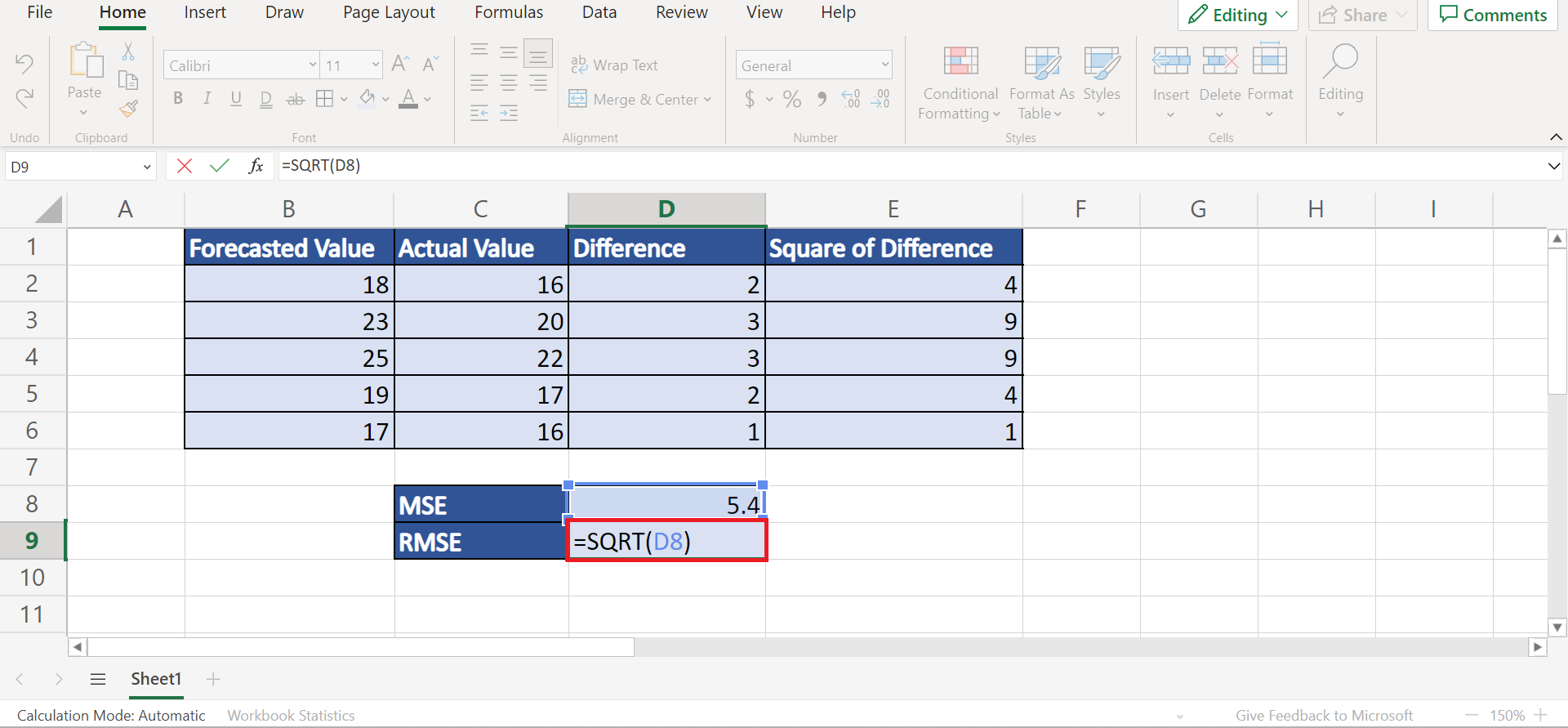
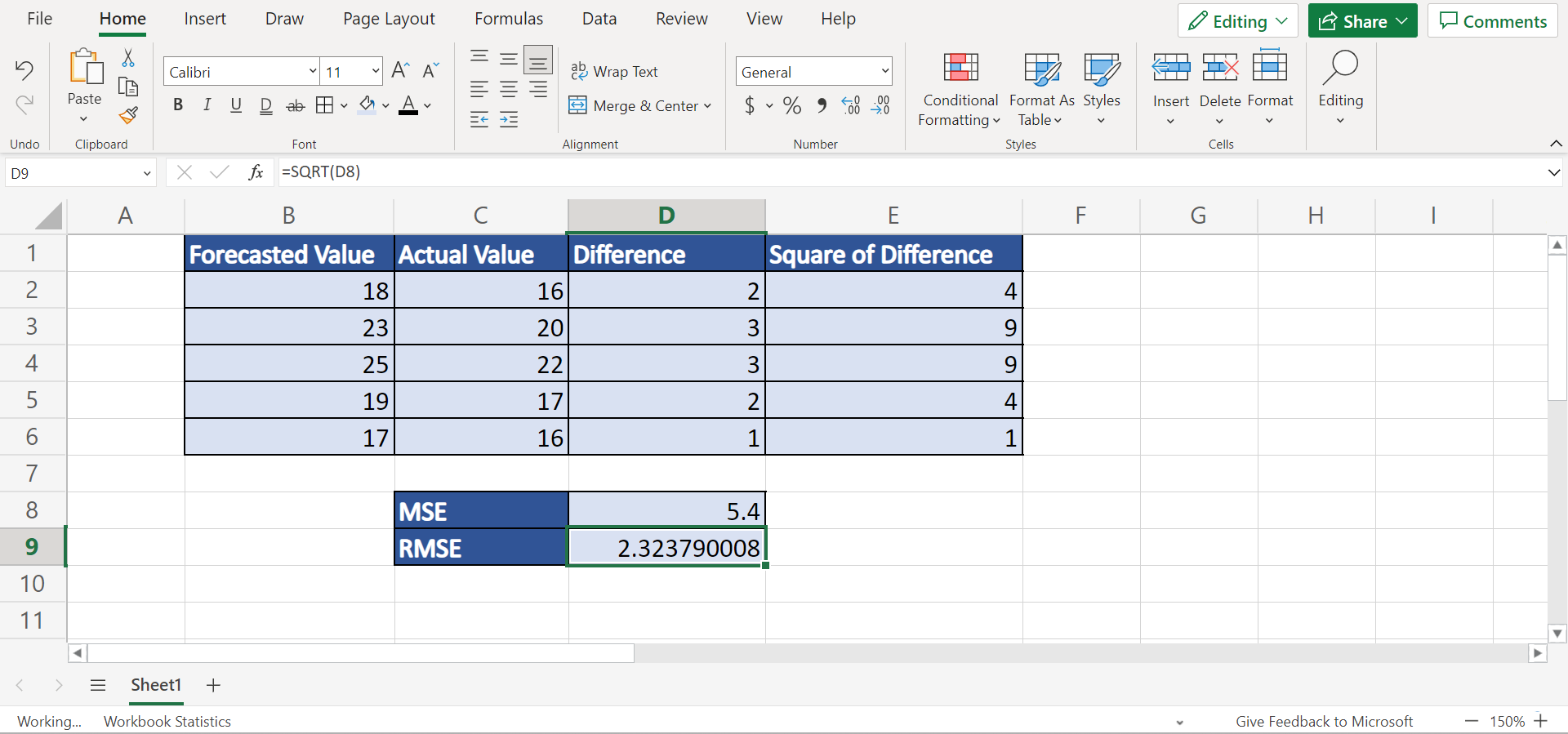
6. Lastly, we will calculate the root mean square error. To do this, we will type in the formula “=SQRT(D8)”. Then, we will press the Enter key to return the result.
7. And tada! We have successfully calculated the root mean square error in Excel.
How to Calculate Root Mean Square Error in Excel using the RMSE Formula
Lastly, we can simply utilize the root mean square error formula in Excel using the SQRT, SUM, and COUNT functions. And the formula to calculate the root mean square error is = √[ Σ(Pi – Oi)2 / n ] wherein Σ represents the sum and Pi refers to the forecasted value for the ith observation in our data set.
Additionally, the Oi in the formula refers to the actual value for the ith observation in our data set. Lastly, n is referring to the sample size.
To do this, simply follow the steps below.
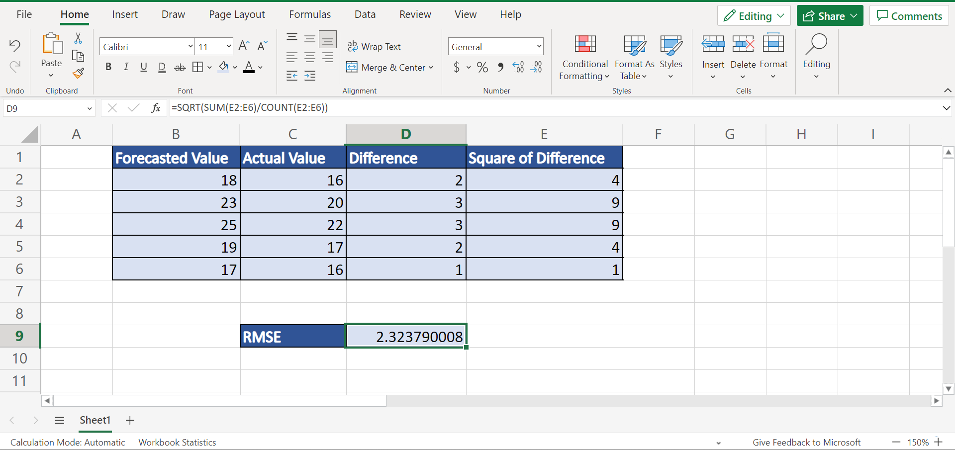
1. Firstly, we can simply input the formula “=SQRT(SUM(E2:E6)/COUNT(E2:E6))”. Then, we will press the Enter key to return the result.
2. And tada! We have successfully used the RMSE formula in Excel.
You can make your own copy of the spreadsheet above using the link attached below.
And that’s pretty much it! We have successfully explained how to calculate the root mean square error in Excel using three simple and easy methods. Now you can simply choose any method that works best for you and use it in your work whenever you need to obtain the root mean square error.
Are you interested in learning more about what Excel can do? You can now use the SUMSQ function and the various other Microsoft Excel formulas available to create great worksheets that work for you. Make sure to subscribe to our newsletter to be the first to know about the latest guides and tutorials from us.


