How to Convert Multiple Rows to Columns and Rows in Excel

This guide will show you how you can convert multiple rows to columns and columns to rows in Excel.

This action is known as transposing a range or table. We’ll look into two ways we can transpose a table in Microsoft Excel.

Let’s take a look at a quick example where we can transpose a range.

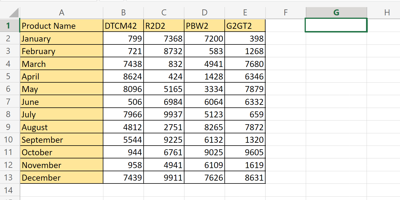
You have a range of values that correspond to monthly sales. Each row corresponds to a month and each column corresponds to a particular category of items. 

You’ve received an instruction that your manager prefers that each column should be a different month, with the categories being arranged per row. Is there an easy way to do this?

We can use either the Paste Transpose option and the TRANSPOSE() function to do this task. The Paste Transpose option is helpful if you want to quickly convert a table to its transposed form. The TRANSPOSE function, on the other hand, is dynamic. This means that you can make changes to the original table and have it reflected in the transposed copy created by the function.

If you find that it makes more sense to rotate a table so that the rows are columns, you should try transposing the range. Let’s learn how to transpose a table ourselves in Excel and later test out the function with actual values.

A Real Example of Using the TRANSPOSE function

Let’s take a look at a real example of transposition being used in an Excel spreadsheet.

In the example below, we have two tables with the same data. The first table has each row correspond to a different month, while each column corresponds to a product name. The second table is a rotated form of the first table’s data. Each row now corresponds to a product name and each column refers to a month.

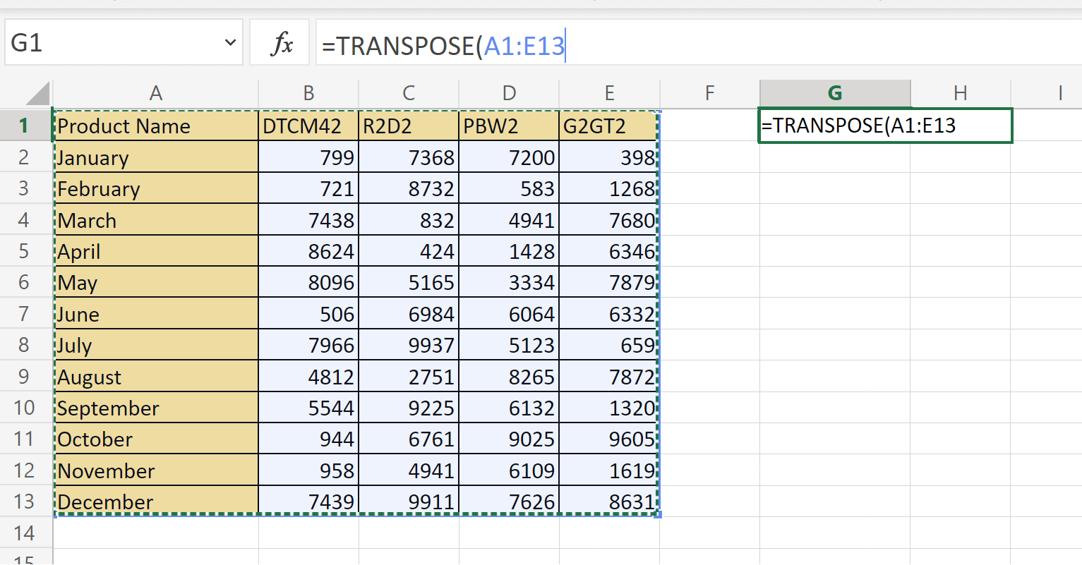
To get the values in the second column, we just need to use the following formula in cell G1:

=TRANSPOSE(A1:E13)

The TRANSPOSE function can also be used with other formulas. In the example below we used the FILTER function on the range A2:A6 to get the values less than 30. We then used the TRANSPOSE function to convert the vertical range into a horizontal range.

To get the values in row 8, we used the following formula:

=TRANSPOSE(FILTER(A2:A6,A2:A6<30))

You can make your own copy of the spreadsheet above using the link attached below. 

If you’re ready to try out transposing data in Excel, follow our step-by-step guide in the next section!

How to Convert Multiple Rows to Columns and Rows in Excel

This guide will show you each step that’s needed to start transposing data in your spreadsheet. You’ll learn how we can use both the Paste Transpose and TRANSPOSE function in Excel to rotate a range.

Follow these steps to start using the Paste Transpose option:

1. First, identify which range you would like to transpose. In the example below, we want to transpose the range A1:E13. This means that each column should indicate a month and each row should belong to a particular product name.
   
   
2. Next, select the entire range that you want to transpose. Type Ctrl + C to copy your selection.
   
   
3. In another cell in your sheet, right-click and select the Transpose icon under the Paste Options.
   
   
4. You should now have the transposed range in your spreadsheet. You can now delete the original table if needed.
   
   

Next, we’ll show you how you can use the TRANSPOSE function in Microsoft Excel.

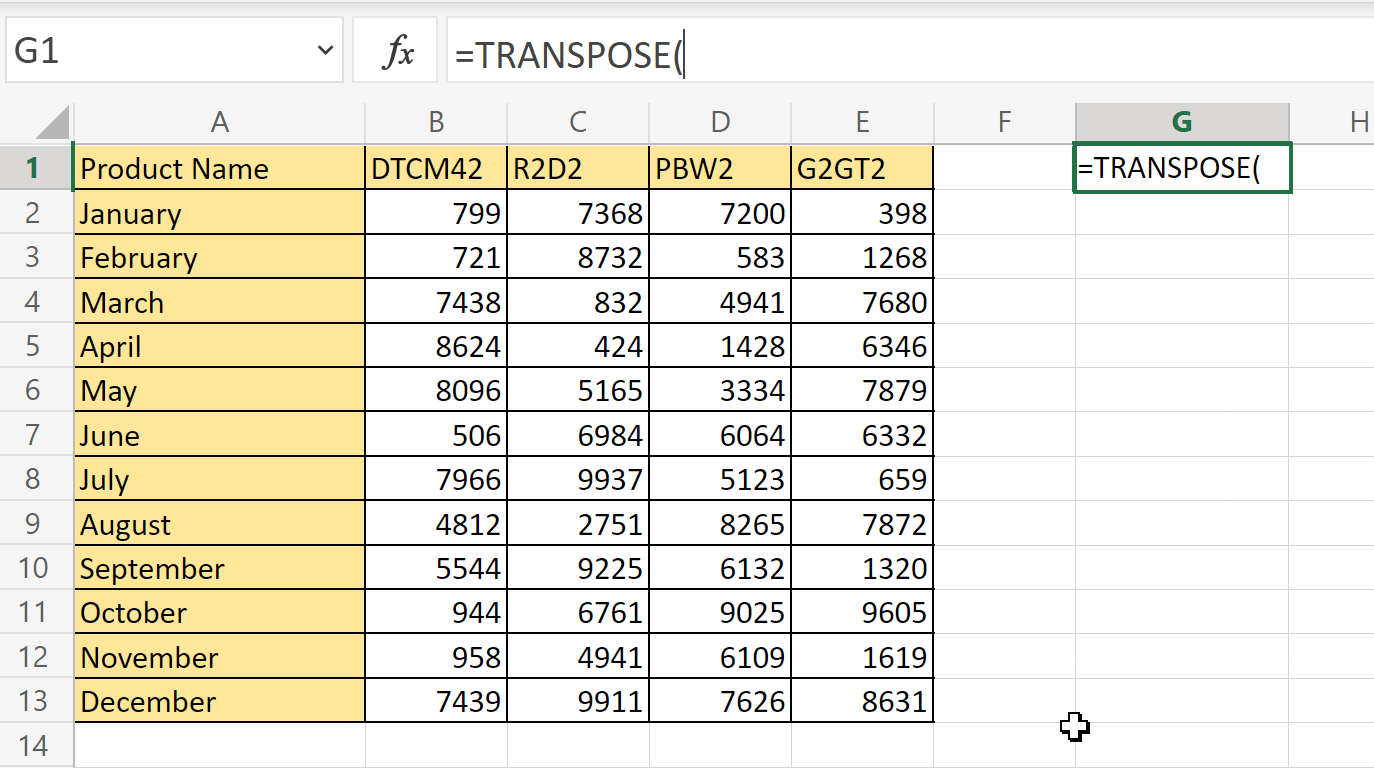
1. The TRANSPOSE function does not change the original table. Instead, it creates a transposed copy of the source table. In this example, we’ve selected the cell G1 to have our TRANSPOSE formula.
   
   
2. Next, type out “=TRANSPOSE(“ in the formula bar to begin the function.
   
   
3. Type in the range you want to transpose as an argument. In this example, we want to transpose the cell range A1:E13.
   
   
4. Hit the Enter key to return the transposed table.
   
   

Frequently Asked Questions (FAQ)

1. What happens if my table includes formulas?
   If your data includes formulas, Excel will automatically update them to match the new placement of each cell. 
2. Should I transpose my data or use a PivotTable?
   Transposing is best used if you only intend to switch two variables as rows and columns.
   It’s also better to use a PivotTable if you intend to frequently change the way you want to see your data. PivotTables make it easy for you to select which fields you want to view as either rows or columns.

That’s all you need to remember to start transposing your data in Excel. This step-by-step guide shows how easy it is to rotate a table so that your rows become columns and vice versa.

Transposing tables is just one of many features Excel has to manipulate your spreadsheet. With so many other Excel functions out there, you can surely find one that can help you out.

Are you interested in learning more about what Excel can do? Make sure to subscribe to our newsletter to be the first to know about the latest guides and tutorials from us. 

Get emails from us about Excel.

Our goal this year is to create lots of rich, bite-sized tutorials for Excel users like you. If you liked this one, you'd love what we are working on! Readers receive ✨ early access ✨ to new content.

Subscribe