How to Create Hyperlink to VLOOKUP Output Cell in Google Sheets

To create a hyperlink to VLOOKUP output cell in Google Sheets is useful if you want to quickly jump to that relevant cell in the lookup table just by clicking the VLOOKUP output cell.

In our previous article, you’ve learned how to VLOOKUP multiple columns in Google Sheets and now you will learn how to create a hyperlink to VLOOKUP the output cell.

Here’s an example: Let’s say you are a teacher and have a list of all your students with their grades from several subjects. And now, you would want to know what grades have some of your students got at one particular subject. We will use the VLOOKUP function to check the grade each of those students has got 📕✏

But what if now you would also want to check grades from other subjects for those students who have obtained an A at that one particular subject? We will create a hyperlink to VLOOKUP output cell (the grade A at that one particular subject) to quickly jump to that relevant cell (the student’s name) in the lookup table just by clicking the VLOOKUP output cell.

But how do we do that?

Simple. The VLOOKUP function needs the search_key (the student’s name), range to search, and the index (column number of the particular subject) to work.

Before showing you how to create a hyperlink to VLOOKUP output cell in Google Sheets, let’s first take a look at the anatomy of the VLOOKUP function.

The Anatomy of the VLOOKUP Function

The syntax (the way we write) the VLOOKUP function is as follows:

=VLOOKUP(search_key, range, index, [is_sorted])

Let’s break this down to better understand the syntax of the VLOOKUP function and what each of these terms means:

• = the equal sign is how we begin any function in Google Sheets.
• VLOOKUP() is our function. To make it work, we must provide the following attributes – search_key, range, and index.
• search_key is the value we are searching for within the range.
• range is the range/array to consider when searching for the search_key.
• index is the column number of the value to be returned (the first column in the range is numbered ‘1’).
• [is_sorted] is optional, and it is TRUE by default. It indicates whether the column to be searched is sorted, and is mostly recommended to put FALSE (unsorted).

⚠️A few notes you should know when writing your own VLOOKUP function in Google Sheets:

1. The search_key must be from the first column of the range.
2. Only the first column in the range will be searched. There is a workaround if you want to search other columns.
3. If [is_sorted] is set to TRUE (sorted), the formula will return the nearest match (< or = to the search_key). When all values in the search column are > the search key, the formula will return #N/A error.
4. If [is_sorted] is set to FALSE (unsorted), the formula will return the exact match. When there are multiple matches, the value from the first found row will be returned. If there is no match, the formula will return #N/A error.
5. To make the cells with no result blank instead of returning the #N/A error, you should simply wrap the VLOOKUP formula with IFNA function.

How to Create Hyperlink to VLOOKUP Output Cell in Google Sheets

Let’s take a look at the example below and learn how to create a hyperlink to VLOOKUP output cell in Google Sheets, step-by-step.

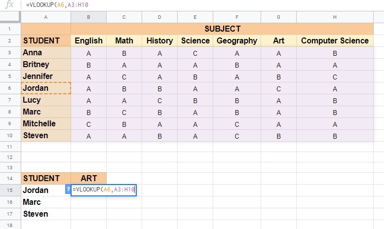
1. Click on the cell B15 to make it active. Type the equal sign ‘=’ to start off the function, and start typing the name of the function, which is VLOOKUP. As you begin typing, a box with the auto-suggested functions that start with ‘V’ will pop-up. You can select the VLOOKUP function by clicking on it, just make sure you click on the right one or close it and ignore it.

2. Then, we will need the search_key (the value we are searching for within the range). In this example, we will use the names of our male students (Jordan – A6, Marc – A8, Steven – A10) as our search_key. After the opening bracket, enter our first search_key, which is A6.

3. Then, we will need the range to consider when searching for the search_key. Enter a comma ‘,’ to act as a separator, and enter our range, which is A3:H10.

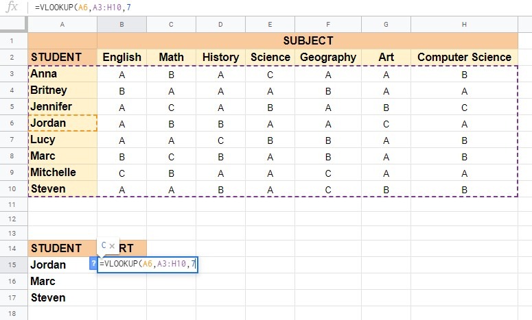
4. And finally, we will need the index (the column number of the value to be returned). Since the first column in the range is numbered ‘1’, the column of the value to be returned (grade at the art class) will be ‘7’. Enter a comma ‘,’ and enter number ‘7’.

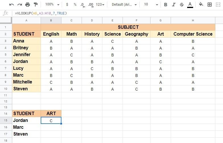
5.  Since our column to be searched is sorted, we will enter a ‘,‘ and TRUE. To close the function, enter the closing bracket ‘)‘ or hit the Enter key on your keyboard. The result in cell B15 should be C.

6.  This is the formula we will use to VLOOKUP Jordan’s grade. We will have to change the search_key for Marc and Steven. For Marc paste =VLOOKUP(A8,A3:H10,7,TRUE) in cell B16 and for Steven paste =VLOOKUP(A10,A3:H10,7,TRUE) in cell B17.

7.  Now, when we know which of our male students has an A at the Art class, we will have to create a hyperlink to the VLOOKUP output cell so we can quickly jump to that relevant cell in the lookup table and look at his other grades. For this, we will need the cell address of the VLOOKUP output cell.

8.  To get the cell address, we should enclose the VLOOKUP formula with the CELL function =CELL(“address”,VLOOKUP(A8,A3:H10,7,TRUE)). Click on the cell C16 and paste the formula.

9.  This will return the cell address as $G$8. But we only need the cell reference G8, without the dollar signs. To remove the dollar signs, we should use the nested SUBSTITUTE formula =SUBSTITUTE(CELL(“address”,VLOOKUP(A8,A3:H10,7,TRUE)),”$”,””). Click on the cell D16 and paste the formula.

10.  Now we need to create a dynamic URL in Google Sheets, which will help us to create a dynamic hyperlink to VLOOKUP output cell. Right-click on any cell and choose ‘Get link to this cell’ from the list. The link will be copied to the clipboard. Paste the copied link in any blank cell, and you will get a URL like this https://docs.google.com/spreadsheets/d/1e9W3RyVEODxgWFfkdf-RpXkySOUtyjIWRmT2C77Knfg/edit#gid=0&range=A1

11.  Remove the part of the link after the equation sign and enclose the URL within double-quotes“https://docs.google.com/spreadsheets/d/1e9W3RyVEODxgWFfkdf-RpXkySOUtyjIWRmT2C77Knfg/edit#gid=0&range=”

12.  Place an ampersand sign ‘&’ at the end of the link and insert the formula after it“https://docs.google.com/spreadsheets/d/1e9W3RyVEODxgWFfkdf-RpXkySOUtyjIWRmT2C77Knfg/edit#gid=0&range=”&
    SUBSTITUTE(
    CELL(“address”,VLOOKUP(A8,A3:H10,7,TRUE)),”$”,””)

13.  Now we have all we need to create a hyperlink to VLOOKUP output cell in Google Sheets. The syntax (the way we write) the HYPERLINK function is as follows =HYPERLINK(URL, [link_label]).

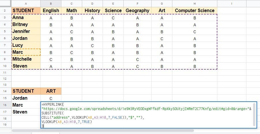
14.  We will replace the URL with the URL we’ve just created, and the link_label with our VLOOKUP formula we used to find Marc’s grade at the Art class.=HYPERLINK(
    “https://docs.google.com/spreadsheets/d/1e9W3RyVEODxgWFfkdf-RpXkySOUtyjIWRmT2C77Knfg/edit#gid=0&range=”&
    SUBSTITUTE(
    CELL(“address”,VLOOKUP(A8,A3:H10,7,FALSE)),”$”,””),
    VLOOKUP(A8,A3:H10,7,TRUE)
    )

15.  Click on the cell B15 and paste the above formula instead of the VLOOKUP formula that is already there. Marc’s grade at the Art class will now be hyperlinked.

16.  You can now click on it and quickly jump to that relevant cell in the lookup table.

You can give it a try yourself by making a copy of the spreadsheet using the link below:

You can now use VLOOKUP function together with the other Google Sheets formulas to create even more powerful formulas that will help you sort and filter your data. 🙂