How to Delete and Shift Cells Left in Google Sheets

This guide will explain how you can use a formula to delete and shift cells to the left in Google Sheets.

We are using the FILTER function to perform this task for individual rows. We will also show how to perform this using an ArrayFormula.

Let’s take a look at a quick example of a scenario where we might want to delete and shift cells to the left.

Suppose you have a dataset containing customer feedback for a restaurant. Each column corresponds to a particular aspect of the business. For example, one column is for feedback regarding the establishment’s food quality. Another column corresponds to their satisfaction with waiting time or ambiance. If the customer has no remarks for a particular aspect, they may leave it blank.

You want to remove these blank answers from the final table. We will label each column as remark_1, remark_2, and so on. How can we delete the blank cells and shift the remaining cells to the left in Google Sheets?

We can use the FILTER function on each row to remove blank cells. We may also use the SPLIT and TRANSPOSE functions to determine which cells are empty. In the next section, we’ll explain how each method works.

Now that we know when to use these formulas, let’s dive into how they work on an actual sample spreadsheet.

A Real Example of Deleting and Shifting Cells Left in Google Sheets

Let’s look at a real example of how Google Sheets functions help delete and shift cells to the left.

In the example below, we’ve used a FILTER function for each row to remove blank cells between values. For example, the value of 23 in row 3 has been shifted to the left in the second table. 

To get the values in Column C, we’ll need to use the following formula:

=IFNA(FILTER(A2:D2,A2:D2<>""),"")

The FILTER function allows you to return a range of cells filtered to meet certain criteria. In the formula above, we used the FILTER function to take out blank values. We use the IFNA function to handle the #N/A error that may happen if the entire row is blank.

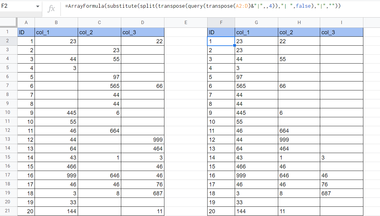
Users may prefer to use an ArrayFormula instead to process the entire table using a single formula:

=ArrayFormula(SUBSTITUTE(SPLIT(TRANSPOSE(QUERY(TRANSPOSE(A2:D)&"|",,4)),"| ",FALSE),"|",""))

In the formula above, we use the TRANSPOSE function and the ‘|’ symbol to create a delimited string for each row. For example, the formula converts the first row to the string ‘1| 23| | 22|’. Using the SPLIT function, the blank values can be ignored if we use the string ‘| ‘ as a delimiter. We can then use the SUBSTITUTE formula to remove any remaining ‘|’ characters.

You can make your own copy of the spreadsheet above using the link attached below. 

If you’re ready to try out these formulas in Google Sheets, let’s begin writing it ourselves!

How to Delete and Shift Cells Left in Google Sheets

This section will explain each step needed to start using Google Sheets formulas to delete and shift values to the left in your spreadsheet. 

Follow these to start using the FILTER function:

1. First, recreate the original table in another part of the sheet. In the example below, we’ve duplicated the table headers in the range A1:D21.
   
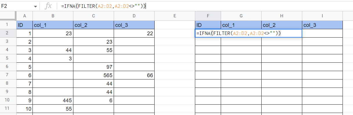
2. Next, we’ll use our FILTER function to duplicate the values in the first row of the table. We wrap the FILTER function with an IFNA function in case the entire row is blank. In our example, we’ll place our FILTER function in cell F2.
   
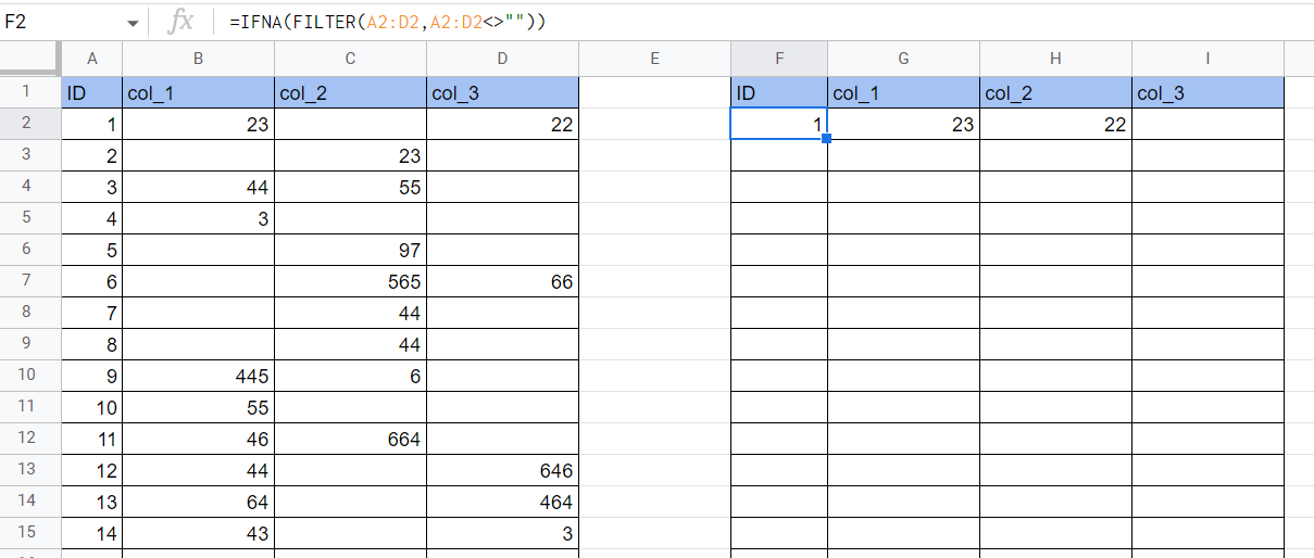
3. Hit the Enter key to evaluate the function. The example below shows that the values 23 and 22 are now shifted to the left. The FILTER function successfully removed the blank cell between these two values.
   
4. Use the Fill Handle tool to apply the formula to the rest of the table. We should now have a table with no blank cells between values of the same row.
   
5. The second table is currently dynamic and will change if we modify the values in the original table. First, select the entire table and press Ctrl + C to convert these formulas to values. While the table is still selected, press Ctrl + Shift + V.
   
6. Your second table should now consist of only numerical values. You may delete the original table safely.
   
7. You can also use an ArrayFormula to process the entire table. Simply use the ArrayFormula seen in the last section. Ensure that the cell range used for the innermost TRANSPOSE function is the original table’s range.
   
   

That’s all you need to remember to start using formulas to delete and shift cells to the left in Google Sheets. This step-by-step guide has shown how to use an ArrayFormula to ignore cells with blank values. We’ve also explained how the FILTER function can be used to remove blank cells in each row.

Deleting and shifting cells left is just one way you can use the FILTER function in Google Sheets. With so many other Google Sheets functions out there, you can surely find one that fits best with your workflow.

Are you interested in learning more about what Google Sheets can do? Make sure to subscribe to our newsletter to be the first to know about the latest guides and tutorials from us. 

Get emails from us about Google Sheets.

Our goal this year is to create lots of rich, bite-sized tutorials for Google Sheets users like you. If you liked this one, you'd love what we are working on! Readers receive ✨ early access ✨ to new content.

Subscribe