This guide will discuss how to find the weighted moving averages in Excel.
Since it has several built-in functions and tools, Excel is a popular tool for performing complex and time-consuming calculations. For instance, we can easily calculate moving averages in Excel.
So a moving average is often used to emphasize recent data values. Furthermore, it is a common technique used to smooth out time-series data to reduce the noise or effects of random and short-term fluctuations.
Using the moving average, we can easily find the pattern or trend in the data set. Additionally, there are three types of moving averages. Firstly, we have the simple moving average, the average of the data values in the given time period.
Secondly, we have the weighted moving average, which considers the recent data values to be more important or have more weight than earlier data values. In this case, the weighted moving average assigned more weight to recent data values and less weight to earlier data values.
Lastly, the exponential moving average is a type of weighted moving average wherein a greater weight is given to the most recent data value, and it decreases exponentially for the older data values.
However, we will only focus on finding the weighted moving average in Excel. Since the weighted moving average assigns greater weight to more recent data values, this is more beneficial to use than the simple moving average.
Additionally, finding the weighted moving average of our data set can give us a more accurate idea of the pattern, especially if our data set is trending in a specific direction.
Let’s take a sample scenario wherein we need to find the weighted moving averages in Excel.
Suppose you have a sales report containing the number of sales for each time period. And you want to present the sales trend for the given time periods. However, you want to emphasize the data values from the more recent time periods. So you opted to find the weighted moving average of your data set.
Great! Now we can move on to a real example of finding the weighted moving averages in Excel.
A Real Example of Finding Weighted Moving Averages in Excel
Let’s say we have a data set containing two columns. Firstly, we have a column for the time period of each sale. And the second column contains the number of sales made for each time period. So our initial data set would look like this:

Although we want to present the sales trend in our data set, we also want to give more weight to the more recent sales time period. In this case, we will utilize the weighted moving average to find the trend in our data set.
So the weighted moving average will simply take the average of a specific number of the previous time periods to come up with an average value for the given period while giving more weight to the more recent time periods.
When finding the weighted moving average, there are two factors we can adjust or change according to our preference or situation. Firstly, we can adjust the number of previous periods used. In this case, we will be using three previous periods. But, we can use four or five previous periods.
Essentially, the more time period we utilize in our calculations, the smoother the weighted moving average line trend will be. Secondly, we can also adjust the weights assigned to each time period. In this case, we will assign the weights 0.6, 0.3, and 0.1.
However, we can assign any weight combination if the weights add up to 1. When we assign a greater weight to the most recent period, the weighted moving average line will be less smooth.
To find the weighted moving average of our data set, we first need to decide how many previous time periods we will use in our weighted moving average calculation. In this case, we will utilize three time periods.
Then, we need to assign weights to each time period. For example, we will assign the weights 0.6, 0.3, and 0.1 to the three previous time periods. In this case, the most recent time period will get 0.6, and the previous time period before that will receive 0.3, while the two time periods back will get 0.1.
Next, we can proceed to calculate the weighted moving average for each period. So we will first multiply the number of sales of each time period by their assigned weight. Then, we will get the sum of all the products from the three time periods.
Afterward, we can insert a line chart to visually present the actual number o sales or each time period compared to the weighted moving average. So our final data set would look like this:

You can make your own copy of the spreadsheet above using the link attached below.
Amazing! Now we can move on and dive into the process of how to find the weighted moving averages in Excel.
How to Find Weighted Moving Averages in Excel
In this section, we will discuss the step-by-step process of how to find the weighted moving averages in Excel. Furthermore, each step has detailed instructions and pictures to help you along the way.
To apply this method, simply follow the steps below.
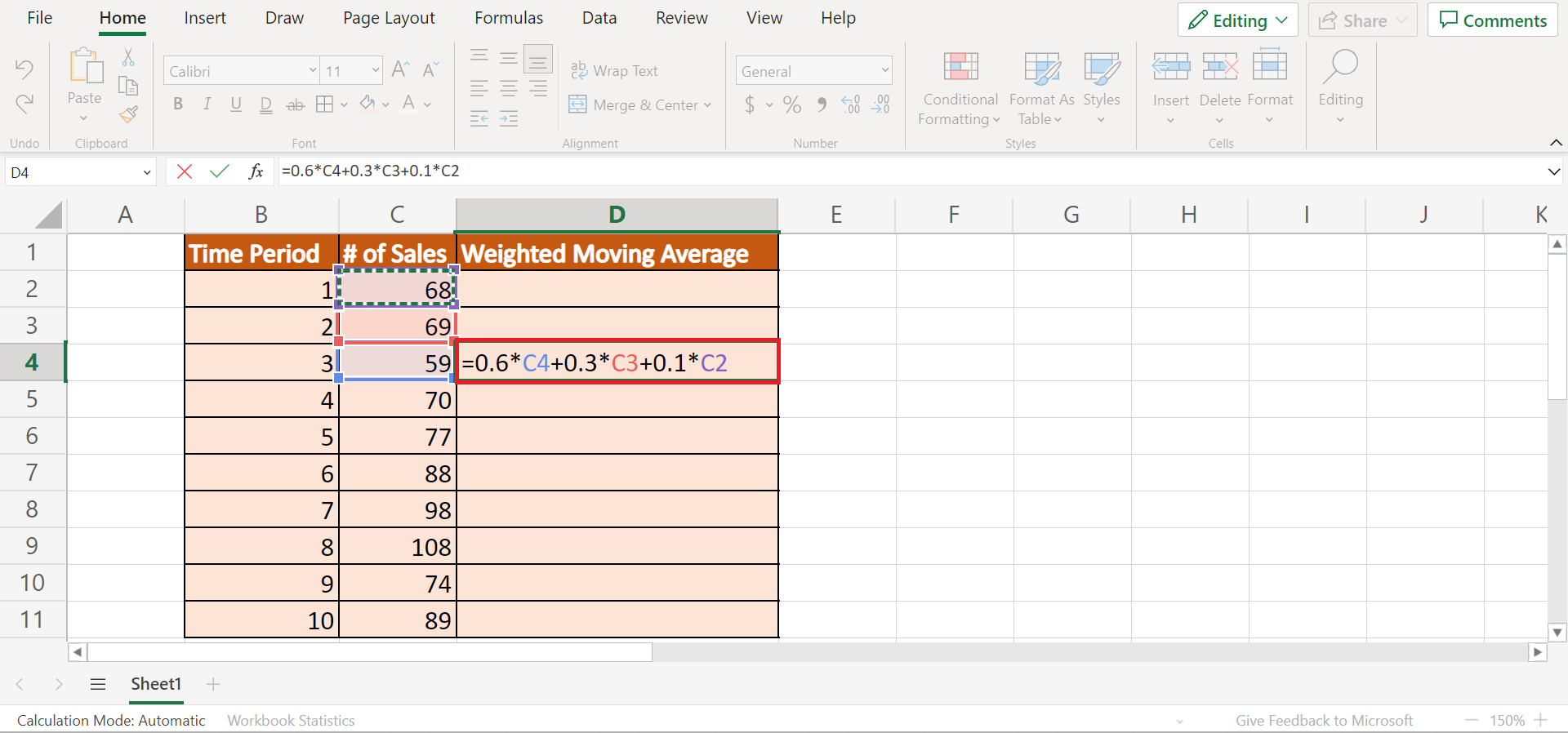
1. Firstly, we need to decide the two factors in our calculation: the number of previous periods and the weights for each time period. In this case, we have included three time periods in our calculation. Moreover, we have decided to assign 0.6, 0.3, and 0.1 as the weights for the time periods.
Since we decided to use three previous time periods, we will start to calculate the weighted moving average from the first three rows in the data set. So we will input the formula “=0.6*C4+0.3*C3+0.1*C2”. Lastly, we will press the Enter key to get the result.
2. Secondly, we will drag down the Fill Handle tool to copy and apply the formula to the other cells.

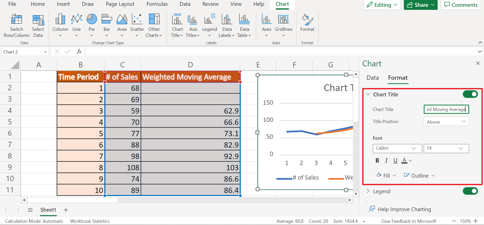
3. Afterward, we can insert a line chart to visualize our weighted moving average compared to the actual values in the data set. To do this, we will select the # of Sales column and the Weighted Moving Average column.
Then, we will go to the Insert tab and select Line. From the dropdown menu, we will choose the Line icon in the 2-D Line section.

4. Once the line chart appears, we can customize it according to our preferences. To do this, we can simply right-click and select Format.

5. Next, we can now format the chart. Let’s say we want to change the chart title. To do this, we can simply head to the Format section and click the dropdown arrow beside Chart Title. In this case, we will change the chart name to “Weighted Moving Average”.
6. And tada! We have successfully found the weighted moving averages in Excel.
And that’s pretty much it! We have discussed the step-by-step process of how to find the weighted moving averages in Excel. You can apply this simple and easy method to your work whenever you need to find the trend in your data set using the weighted moving average.
Are you interested in learning more about what Excel can do? You can now use the various other Microsoft Excel formulas available to create great worksheets that work for you. Make sure to subscribe to our newsletter to be the first to know about the latest guides and tutorials from us.