This guide will explain how to highlight a cell or row that displays the current time interval in Google Sheets.
Table of Contents
Given a Google Sheets table containing a sequence of time intervals, you may want to highlight a specific cell or row in that sequence if it matches the user’s current time.
For example, to make a daily schedule more readable, we may want to highlight the row corresponding to the current time. For example, if the current time is 2:45 PM, you would like the 2:30 PM row highlighted and so on. To format our cells, we can use the built-in Conditional Formatting tool and use a custom formula to determine which cells to highlight.
In this guide, we will provide a step-by-step tutorial on how to use conditional formatting in Google Sheets to highlight the current time.
The Anatomy of the XMATCH Function
The syntax of the XMATCH function is as follows:
=XMATCH(search_key, lookup_range, [match_mode], [search_mode])
Let’s look at each argument to understand how to use the XMATCH function.
- = the equal sign is how we start any function in Google Sheets.
- XMATCH() refers to our built-in
XMATCHfunction. This function returns the relative position of an item in an array or range which matches some specified value. - search_key refers to the value to search for. We’ll set this value to the current time rounded down to a specific time interval.
- lookup_range argument refers to the range to consider when searching. This range must be a single row or column.
- match_mode argument is an optional argument that determines how to find a match. By default, the
XMATCHformula returns exact matches. - The search_mode argument is another optional argument which controls the direction and method to search. By default,
XMATCHsearches from the first entry to the last.
A Real Example of Extracting Time from DateTime Values in Google Sheets
Let’s explore a simple example where we can use a custom formula and conditional formatting to highlight the current time.
Suppose we have a weekly schedule template where each row corresponds to 30-minute intervals between 9am and 5pm.
The first column will hold the time when the interval starts (9am, 1:30pm and so on) and the succeeding columns will be used to write down specific deadlines or meetings to attend on a specific day of the week.

In the table above, we have a weekly schedule with various cells highlighted to indicate meetings and events for a particular block of time.
We want to highlight the cell in column A that corresponds to the current time. To do this, we can use the following formula:
=XMATCH(FLOOR(MOD(NOW(), 1), "0:30"), A2)
Let’s try to understand what the formula above tries to accomplish.
The NOW function returns the current date and time. We’ll use MOD(NOW(),1) to discard the current date and output just the time component.
Next, we’ll use the FLOOR function to round down the time value to the nearest multiple. In this case, we’ll round down the time component to the nearest 30-minute interval by specifying “0:30”.
Lastly, the XMATCH function takes the output of our FLOOR function and tries to find a match within a specific range.
This custom formula will be used as a criteria for the built-in conditional formatting tool to highlight the cell containing the current time interval.

To highlight the entire row, we can simply replace “A2” with “$A2” instead:
=XMATCH(FLOOR(MOD(NOW(), 1), "0:30"), $A2)

In some cases, the time interval may be different. For example, each value in the sequence may jump ahead in 15-minute intervals or even intervals of an hour.

In the schedule template above, each row represents an hour instead of a 30-minute block. We can modify our earlier formula to account for this new time interval:
=XMATCH(FLOOR(MOD(NOW(), 1), "1:00"), $A2)

Click on the link below to create your own copy of our examples.
Head to the next section to read our step-by-step tutorial on how to highlight the current time in Google Sheets.
How to Highlight Current Time in Google Sheets
- First, select the range containing the time you want to highlight.

In this example, we want to highlight a specific cell in column A if the current time corresponds with the cell’s time time. Note that the range must be in a single column. - Next, we’ll need to access the conditional formatting options.
To access the conditional format rules panel, select Format > Conditional formatting.
- By default, you should see options under the Single color tab. Do ensure that the range under Apply to range corresponds to the range containing time values.

Expand the dropdown menu under Format cells if… and select Custom formula is. In the provided input box, type the following formula: =XMATCH(FLOOR(MOD(NOW(), 1), “0:30”), A2).
You may change “0:30” in the formula above depending on the required time interval. The argument A2 should be replaced with the first cell in the target range. - After setting our custom formula, we should now apply the formatting style. You can choose to format the cell background to a certain color and format how the cell’s text appears. Click on Done to proceed.

For our example we’ll highlight the current time with a gray cell background and bolded text. - The cell corresponding to the current time interval should now be highlighted using conditional formatting.

- To highlight the entire row, simply convert the cell reference from A2 to $A2.

To learn more about applying formatting dynamically in Google Sheets, you can read our post on how to use conditional formatting in Google Sheets.
That’s all for this guide! Don’t forget to check out our library of spreadsheet resources, tips, and tricks for both Google Sheets and Microsoft Excel!