This guide will explain how to do conditional formatting if between two values in Excel.
Since it has several built-in functions and tools, we can easily perform complex tasks in Excel. Excel is a powerful tool for different purposes and situations. For example, we can highlight certain values in our dataset based on different conditions using conditional formatting.
So conditional formatting is an excellent feature in Excel that allows us to easily identify specific values in our data set. Moreover, it is extremely helpful when we need to highlight values in our data set that fit certain conditions or criteria.
In this case, we want to apply conditional formatting for cells if the value falls between two values. Luckily, it is easy for us to perform this task as Excel already has built-in conditional formatting rules we can utilize.
Moreover, we can also create a new rule and apply the AND function to apply conditional formatting between two values.
Let’s take a sample scenario wherein we need to do conditional formatting if between two values in Excel.
Suppose you are a teacher inputting the students’ grades in Excel. And you have set the passing score to 75 and above. So you want to identify the students who failed the test. To do this, you applied conditional formatting for cells with scores between 0 and 74.
Before we move on to a real example of doing conditional formatting if between two values in Excel, let’s learn more about the AND function.
The Anatomy of the AND Function
The syntax or the way we write the AND function is as follows:
=AND()
Let’s take apart this formula and understand what each term means:
- = the equal sign is how we activate any function in Excel.
- AND() is our
ANDfunction. And this function is used to check whether all arguments are TRUE and returns TRUE if all arguments are TRUE. - logical1 is a required argument. So this refers to 1 to 255 conditions we want to test that can either be evaluated as TRUE or FALSE. Furthermore, we can input logical values, arrays, or cell references.
- logical2 is an optional argument. And this refers to 1 to 255 conditions we want to test that can either be evaluated as TRUE or FALSE. So this serves as a supplement to the first required argument.
Great! Now we can dive into a real example of doing conditional formatting if between two values in Excel.
A Real Example of Doing Conditional Formatting if Between Twp Values in Excel
Let’s say we have a data set containing students’ test scores. So we have two columns showing the student’s name and their test score. And our initial dataset would look like this:

For instance, we set the passing score for the test to be 75 and above. Thus, any score between 0 and 74 is considered a failing score. So we want to easily identify the students who failed the test. To do this, we can apply conditional formatting in our data set.
So there are two ways we can apply conditional formatting to our data set to highlight the students who failed the test. Firstly, we can simply use the built-in rule created by Excel. Then, we can choose the between rule to make the condition highlight cells containing scores between 0 and 74.
Secondly, we can also choose to create a new rule and apply the AND function to highlight cells containing scores between 0 and 74. So the AND function will check whether all cells contain a value between 0 and 74. If TRUE, the cell will be highlighted. If FALSE, the cell will remain as is.
Moreover, we can choose different formats, such as font color and cell color, allowing us to customize the formatting with whatever fits the situation. Our final data set looks like this:

You can make your own copy of the spreadsheet above using the link attached below.
Amazing! Now we can proceed and explain the process of how to do conditional formatting if between two values in Excel.
How to Do Conditional Formatting if Between Two Values in Excel
In this section, we will explain the step-by-step process of how to do conditional formatting if between two values in Excel. Additionally, each step contains detailed instructions and pictures to help you along the process.
To apply this method to our work, we can simply follow the steps below.
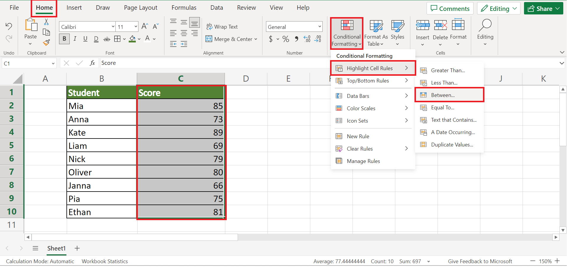
1. Firstly, we need to highlight our data set. Then, we will go to the Home tab and select Conditional Formatting in the Styles section. Next, we will choose Highlight Cells Rules in the dropdown menu. Lastly, we will click Between.
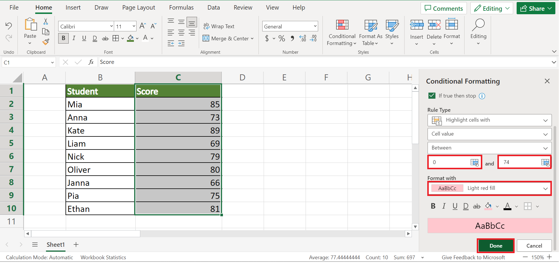
2. Secondly, a pop-up menu will appear at the side where we can input our condition. In this case, we will input “0” as our lower value and “74” as our upper value. Additionally, we can select the format we want to highlight the cells. Lastly, we will click Done to apply the changes.
3. And tada! We have successfully applied conditional formatting if between two values in Excel.

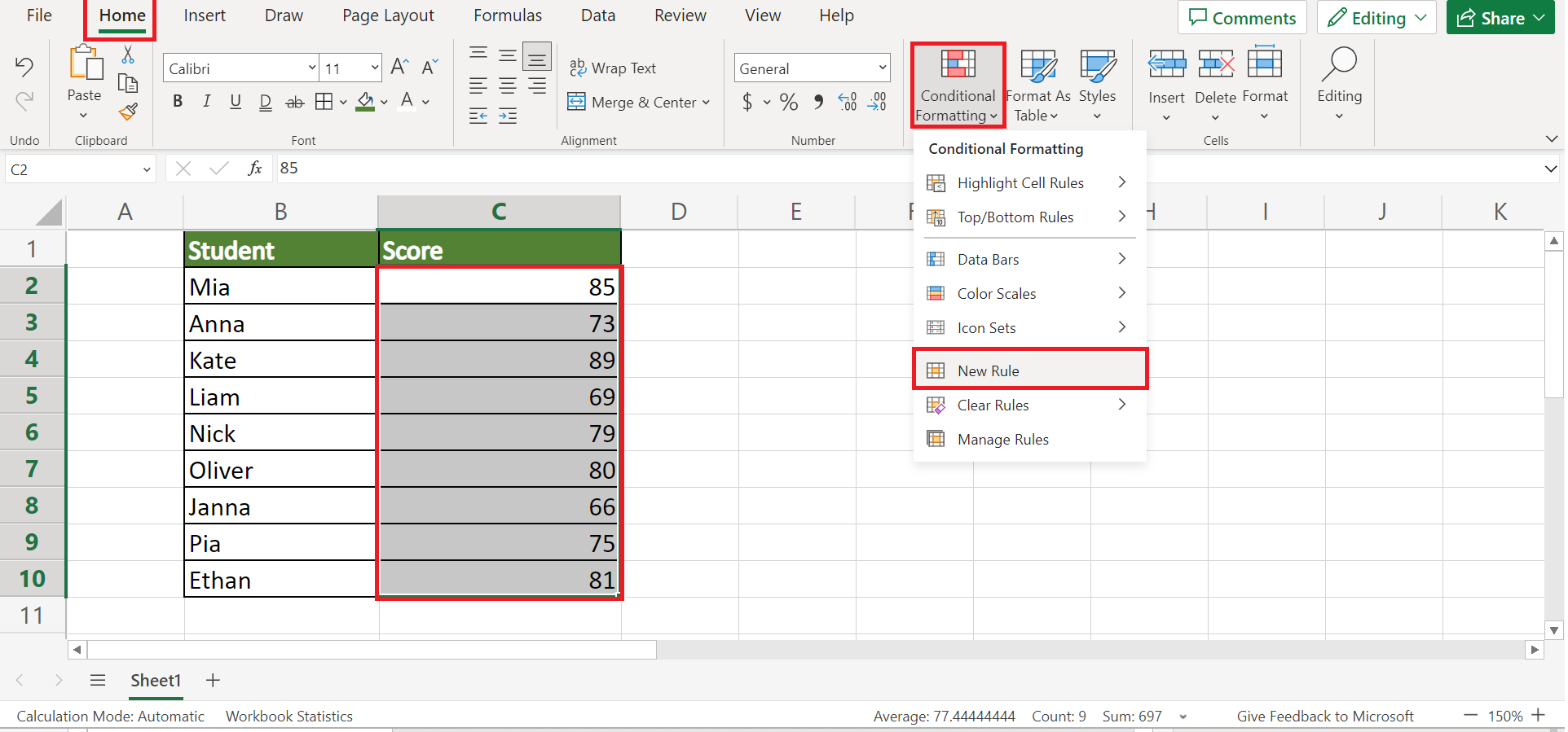
4. Alternatively, we can create a new rule and input a formula using the AND function. To do this, we will select our data set and go to the Home tab. Then, we will click Conditional Formatting. Next, we will select New Rule in the dropdown menu.
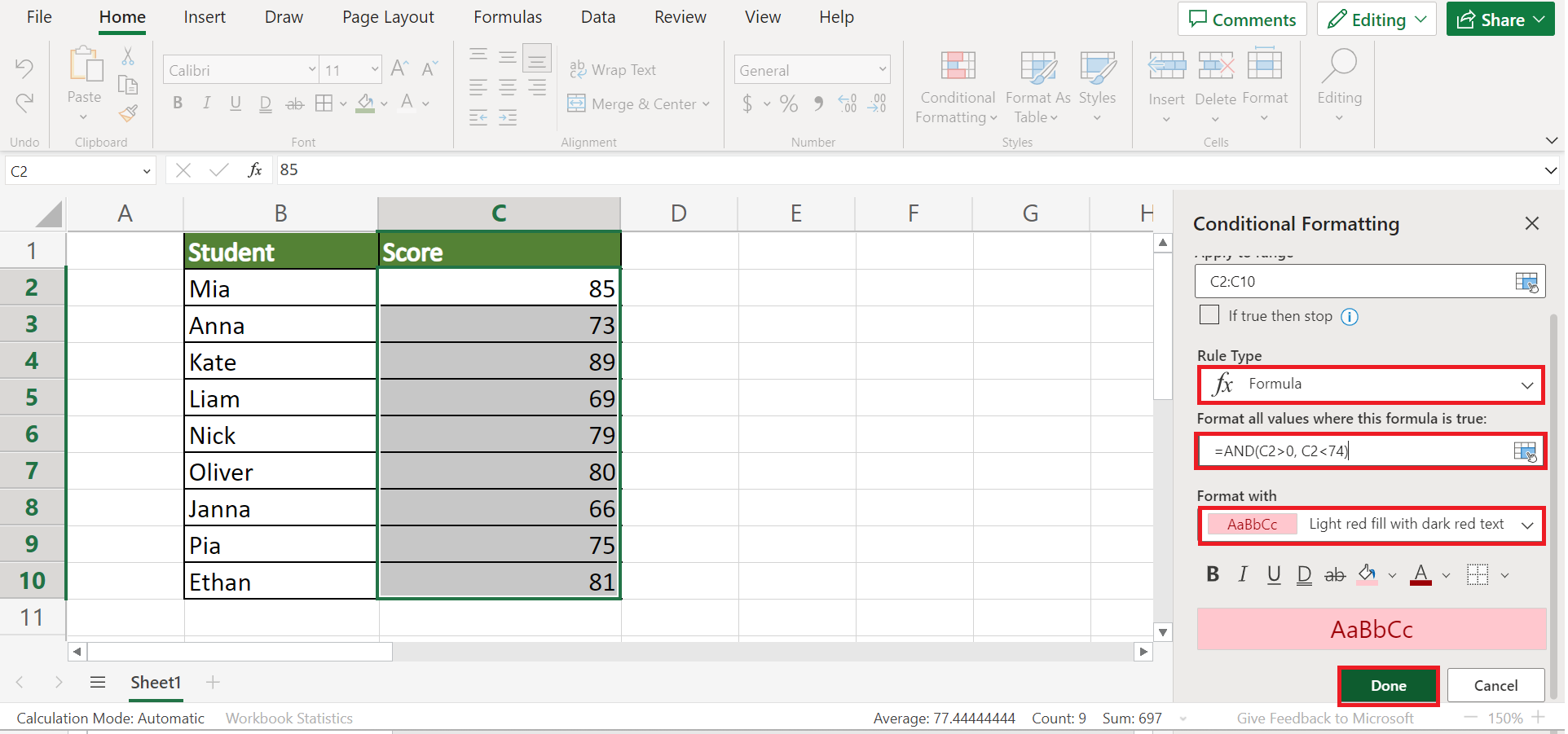
5. In the Conditional Formatting menu that appears at the side, we first have to select Formula in the Rule Type. Next, we will input the formula “=AND(C2>0, C2<74)”. Next, we can select the format we want to apply to the cells. Lastly, we will click Done to apply the changes.
6. And tada! We have successfully created a new rule that highlights cells if between two values in Excel.
And that’s pretty much it! We have successfully explained how to do conditional formatting if between two values in Excel. Now you can choose any of the methods and apply them to your work whenever necessary.
Are you interested in learning more about what Excel can do? You can now use the AND function and the various other Microsoft Excel formulas available to create great worksheets that work for you. Make sure to subscribe to our newsletter to be the first to know about the latest guides and tutorials from us.