The STDEV Function in Google Sheets is useful if you want to find out the standard deviation from the mean for a given set of values.
Meaning, it indicates how much the values of the given set of data spread out from the mean. Like any other statistical function, this is commonly used by professionals in accounting, investing, and economics.
Table of Contents
Similar to the AVEDEV function, the rules for using the STDEV function in Google Sheets are as follows:
- Arguments can be numbers, cell ranges, arrays, or references that contain numbers.
- The function ignores empty cells, and cells that contain text or logical values. However, cells with the value zero are included.
- If you use text, blank cells, error, or Boolean values directly as arguments in the formula, AVEDEV will return an error.
- Likewise, if all your argument values are strings, you are going to get an error.
Let’s take an example.
Please take a look at the scores below:
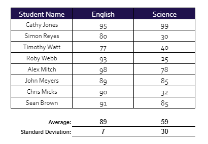
For the English subject, the standard deviation is 7, which means that the most of the students got no more than 5 points from the average. This tells us the consistency of the scores of the students for that subject.
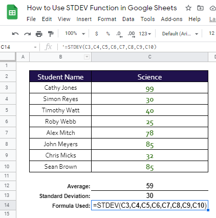
On the other hand, the set of scores for the Science subject has a standard deviation of 30. It shows that there’s a wide spread out of scores, which means that some students performed well and some performed worse than the average.
Let’s have another real-life sample!
Janine is using the standard deviation to determine the volatility of an investment return. A higher standard deviation means a huge dispersion in the average return, which is a risky investment. On the other hand, a lower standard deviation means consistency in the average return, which means a safer and lower risk investment.
Watch out for a more advanced tutorial and examples on how you can use the STDEV function in the coming weeks. Be sure to subscribe to be notified.
Awesome! Let’s begin getting to know more about our STDEV function in Google Sheets.
The Anatomy of the STDEV Function
So the syntax (the way we write) the AVEDEV function is as follows:
=STDEV(value1, [value2,value3,...])
Let’s dissect this thing and understand what each of these terms means:
- = the equal sign is just how we start any function in Google Sheets. It is how Google Sheets understand that we are asking it to either do a computation or use a function.
- STDEV() this is our STDEV function. STDEV will take the values and compute them for the standard deviation.
- value1 is the first value or reference to the range of the dataset.
- value2,value3,… [optional] are the additional values or references to ranges that contain values we need to include in the dataset.
A Real Example of Using STDEV Function
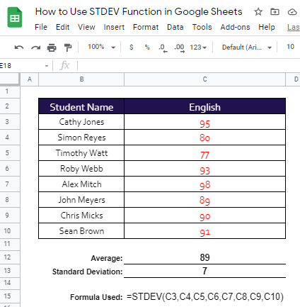
Take a look at our scores example below to see how the STDEV function is used in Google Sheets.

We already know that the standard variation for English and Science are 7 and 30 (rounded off for better data representation), respectively.
What we don’t know is how these two numbers were calculated. Let’s go and analyze!
The standard deviation for the subject English for the given set of scores was derived by using the STDEV function. Please see cell C15 below for the formula used:

While there are 8 scores in the set of values, notice that only 1 argument is used for our STDEV function. Yes, you read it right! The range C3:C10 is treated as 1 argument only. This means that you can still provide another set of constant or another range of cells as a second argument and our STDEV function will compute for the standard deviation for that set of data.
There’s nothing wrong with using 1 cell address as 1 argument in our STDEV function or any other function, for that matter, as the result will still be the same.
However, it is tedious and time consuming, especially if you have multiple cell addresses to use. So, it is advisable and efficient to use cell range, instead.
Let’s have another example:
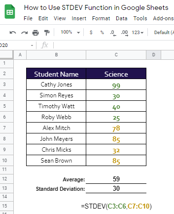
Take a look at C13 for the standard deviation of the given set of scores.
Notice in cell C15 that our STDEV function has two arguments, C3:C6 and C7:C10. It goes to show that, whether we pass our STDEV function 2 different cell ranges as first and second argument, it still treats them as the set of data which it needs to compute the standard deviation from.
You may make a copy of the spreadsheet using the link I have attached below.
How to Use STDEV Function in Google Sheets
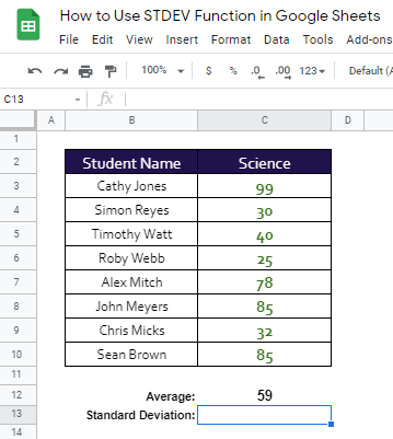
- Click on any cell to make it the active cell. For this guide, I will be selecting C13, where I want to show my result.
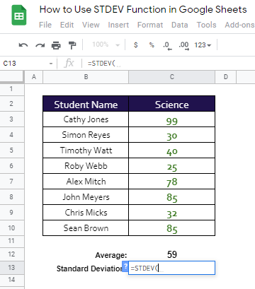
- Next, type the equal sign ‘=‘ to begin the function and then followed by the name of the function, which is our ‘stdev‘ (or ‘STDEV‘, not case sensitive).
- Type open parenthesis ‘(‘ or simply hit Tab key to let you use that function.
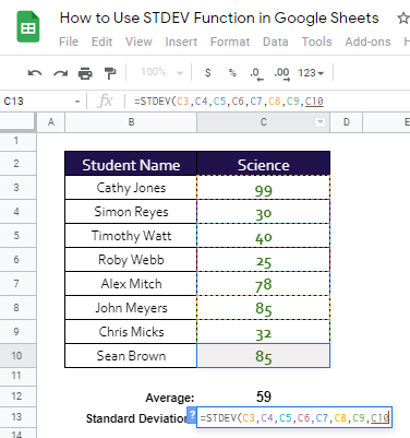
- Now the exciting part! Let’s give our function the argument, which is the list of given values. You may pass a constant data by typing each of the given values after the parenthesis. For this example, I’ll be using the cell address of each value. Type in C3 or the cell address of 99 in our set of scores.

- To let the Google sheet know that we’re done typing our first argument, we should now type in the delimiter or the character that separates each argument on a function. In this case, type comma ‘,’ followed by the next argument, which is the cell C4.

- Separated by the delimiter, the rest of the cell addresses should follow.
- Finally, just hit your Enter or Tab key. The cell C13 is now showing you the result or the return value of the STDEV function.
- Notice that, in our example above, we provided eight arguments, the cell address of each value, to our STDEV function. Alternatively, you can simply use the range of your data, in this case, C3:C10.
- In cell C17, follow steps 1-7. Only this time, we will use the cell range where your set of values is located, C3:C10.

- Check and compare the results in cells C13 and C17. They should be the same.

That’s pretty much it. You can now use the STDEV function in Google Sheets together with the other numerous Google Sheets formulas to create even more powerful formulas that can make your life much easier.