The WEEKDAY function in Google Sheets is useful if you want to give a numerical value to a day in a week of a date.
Meaning the WEEKDAY function can be used in businesses that have different daily rates, highlighting a specific day in a week on your data, or a higher pay during weekends.
Table of Contents
The rules for using the WEEKDAY function in Google Sheets are as follows:
- The data that will be referenced on the WEEKDAY function should either be a cell that contains a date, a function that returns a date like DATE(), or an inputted data in a date format that Google sheets can recognize(e.g. 8/15/1989).
- Dates that are directly passed to the WEEKDAY function should be enclosed with quotation marks.
- The WEEKDAY function does not return a letter (e.g. ‘W’ or ‘M’), an abbreviation (e.g. ‘Sat’ or ‘Sun’), or a full day name (e.g. ‘Tuesday’) of the week. It will return a numerical value ranging from 0 to 6 or 1 to 7, depending on your preference.
Let’s take an example.
One customer stayed in our hotel for a total of five days. He is about to check out today and I need to determine her total bill. The given data is as follows:

Using the WEEKDAY function in Google sheets, I was able to put a value on the specific days the customer checked in as shown in column B. In this case, I use the default type that returns a value between 1 to 7 that starts on Sunday.
What I did after to take advantage of the data provided by the WEEKDAY function, I just had to use the IFS function to determine the equivalent rates, in this case, we had 3 arguments.
First is if the value is less than 6, it is equivalent to the Sun – Mon rates. If the value is exactly 6, then the rate is for Friday. Lastly, if the value is 7, then we use the Saturday rates.
As you can see in column C, I was able to come up with the total bill of $529.95.
Let’s have another example!
John was asked to provide an invoice for his weekly payout. However, the job offers a different pay rate for weekends. Here is the data provided by John:
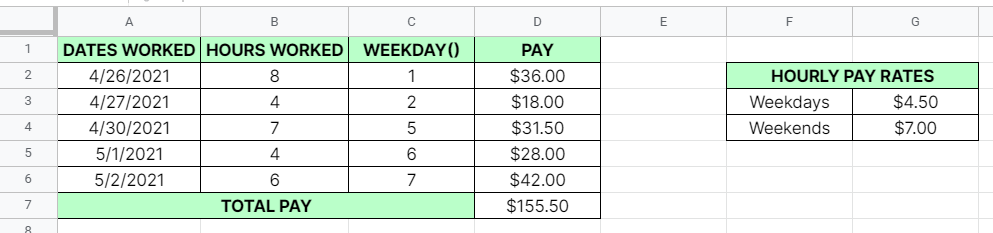
This example is similar to the previous one, except this time, we have to take into consideration the hours worked and the week starts on Monday.
The WEEKDAY function was used this time to put a value on the specific day John worked shown in column B. Although, in this case, John used the 2nd type for numbering the days, this values the days starting from Monday(1) to Sunday(7).
With the data provided by the WEEKDAY function, John just had to multiply the hours worked to the equivalent pay rates using the same process we did in the previous example.
Only this time, we have 2 arguments. If the value is less than six, we will use the weekdays’ hourly pay rates. Otherwise, we will use the weekends’ hourly pay rates. This is shown in column D with the total pay amounting to $155.50
Watch out for a more advanced tutorial and examples on how you can use the WEEKDAY function in the coming weeks. Be sure to subscribe to be notified.
Perfect! Let’s begin getting to know more about our WEEKDAY function in Google Sheets.
The Anatomy of the WEEKDAY Function
So the syntax (the way we write) the WEEKDAY function is as follows:
=WEEKDAY(date, [type])
Let’s dissect this thing and understand what each of these terms means:
- = the equal sign is just how we start any function in Google Sheets. It is how Google sheets understand that we are asking it to either do computations or use a function.
- WEEKDAY() this is our WEEKDAY function. It will return a number representing the day of the week of the date provided.
- date is the first argument that will determine the date you want to reference for the WEEKDAY function.
- type is an optional argument that defaults to 1, this is the argument that determines the numbering system you wish to use as a representation of the weekdays. The most common options are as follows:
- Type 1 counts the day from Sunday, represented by 1, to Saturday, represented by 7.
- Type 2 counts the day from Monday, represented by 1, to Sunday, represented by 7.
A Real Example of Using WEEKDAY Function
Take a look at the example below to see how the WEEKDAY function is used in Google Sheets.

As you can see, in using the WEEKDAY function, we can either reference a particular cell or directly pass our data to the function.
The important thing is that the format of the date we provide is in a format that Google Sheets will recognize. You can also see here that I did not include the second argument type, which defaulted to type 1. That’s why May 8, 2021, a Saturday is, represented by 7.
Let’s have another example!
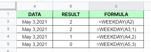
In the example above, we showcase the different type options we can use for the second argument of the WEEKDAY function in Google Sheets.
We used the date May 3, 2021, a Monday, in all of the formulas. As you can see, whether we put 1 as a second argument or not put a second argument at all, it provides the same result.
Why is this so?
Well, that’s because of the default option.
In using 2 as our second argument, we received the result 1 since the count starts on a Monday. Although it also starts on a Monday, the last example gave us 0 as a result since that is where the count starts for type 3.
You may make a copy of the spreadsheet using the link I have attached below.
How to Use WEEKDAY Function in Google Sheets
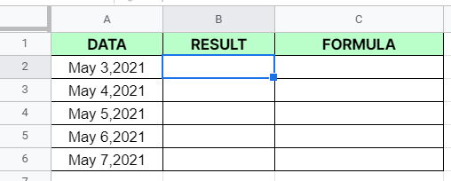
- Simply click on any cell to make it the active cell. For this guide, I will be selecting B2 where I want to show my result.
- Next, type the equal sign ‘=‘ to begin the function and then followed by ‘week‘ (or ‘WEEK‘, not case sensitive).
- You should find that the auto-suggest box appears with the names of the functions that all start with WEEK. You may use your mouse to click on the WEEKDAY or use your down arrow keys to highlight and hit the enter key. Alternatively, you may completely type WEEKDAY and hit the Tab key to let you use that function.

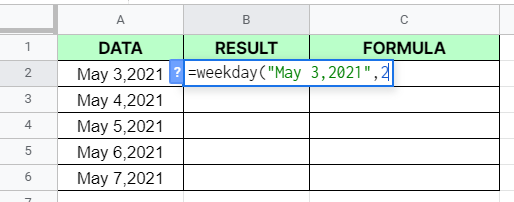
- Now the fun part! Let’s give our function the first argument, which is the date. You may pass constant data by typing the exact date after the parenthesis. Don’t forget to enclose the exact date value to quotation marks (“”).

- To let the Google sheet know that we’re done typing our first argument, we should now type in the delimiter or the character that separates each argument on a function. In this case, type comma ‘,‘ followed by the second argument, which is the [type]. This argument is again optional, you may choose not to put a second argument which will default to type 1, but in this practice, I will be using 2.
- Finally, just hit your Enter or Tab key. The active cell will now show you the result or the return value of the WEEKDAY function.
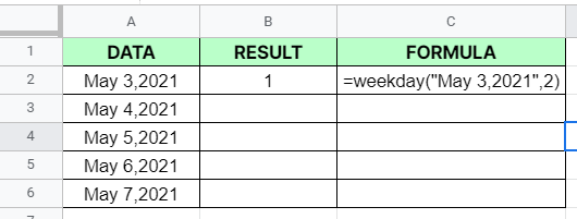
- Notice that in this example, we provided the exact value, constant, as the arguments of our WEEKDAY. Alternatively, this constant can be a variable or simply a cell address of your data.
- Edit your function by changing the first argument into the cell address where your date is located. In this case, type in A2.
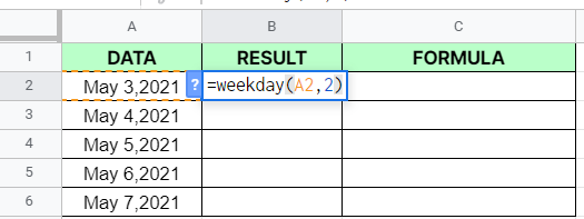
- Copy the formula down to the remaining rows.

That’s pretty much it. You can now use the WEEKDAY function in Google Sheets together with the other numerous Google Sheets formulas to create even more powerful formulas that can make your life much easier.