The IMABS function in Google Sheets returns the absolute value (the modulus) of a complex number.
A complex number is formatted as a string equation “a+bi” or “a+bj” where a and b are real numbers, and i is the symbol for the imaginary number, such that i=√-1 or i2=−1. The coefficient j can also be used to symbolize the imaginary number since in some disciplines since using i can be confusing.
Table of Contents
The formula for IMABS is defined as follows:

Let’s take an example.
I’m trying to get the modulus or absolute value of 2+4i. The real part of my string equation is 2, while the imaginary part is 4. To calculate the absolute value, the formula goes IMABS (2+4i)=√22+42=√4+16= 4.472135955.
Together, let’s learn how to write the IMABS function in Google Sheets.
The Anatomy of the IMABS Function in Google Sheets
The syntax (the way we write) of the IMABS function goes as follows:
=IMABS(inumber)
Let’s dissect this thing and understand what each of these terms means:
- = the equal sign is just how we start any function in Google Sheets.
- IMABS () is our
IMABSfunction. - inumber is the complex value used to calculate the absolute value enclosed in parentheses with no spaces in between characters such as “2+3i”. It could also be a simple numeric value like -3, a reference to a cell with a complex number or a simple value such as B4, or a value returned from the COMPLEX function like COMPLEX(4,3).
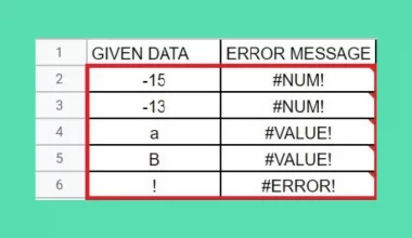
Note that you will get the #NUM! error value if your inumber has an invalid format such as “2+i3”, “j+1”, and “j+i”. It’s also important to remember that the coefficients i or j in the complex number need to be in lower case for the formula to be valid. On the other hand, you will get the #VALUE! error value if your inumber is a logical value.
Real Example of Using the IMABS Function in Google Sheets
Now, let’s take a look at some numbers I’m presenting to see how an IMABS function will look like in Google Sheets with the different valid inumber formats.

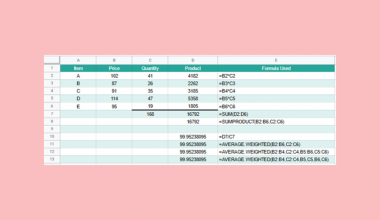
In the table, the IMABS function calculates with the inumbers on column A. As you see, the formula can include fractional values in the real and imaginary parts. Also, the imaginary part can use i or j interchangeably.
Moreover, the function can calculate the absolute value of an inumber that is entered in a cell. And it can return a value with either only the real part or the imaginary part as an inumber.
You can make a copy of the spreadsheet I made using the link attached below:
At this point, I’ll show you how you can do this yourself with comprehensive steps.
How to Use the IMABS Function in Google Sheets
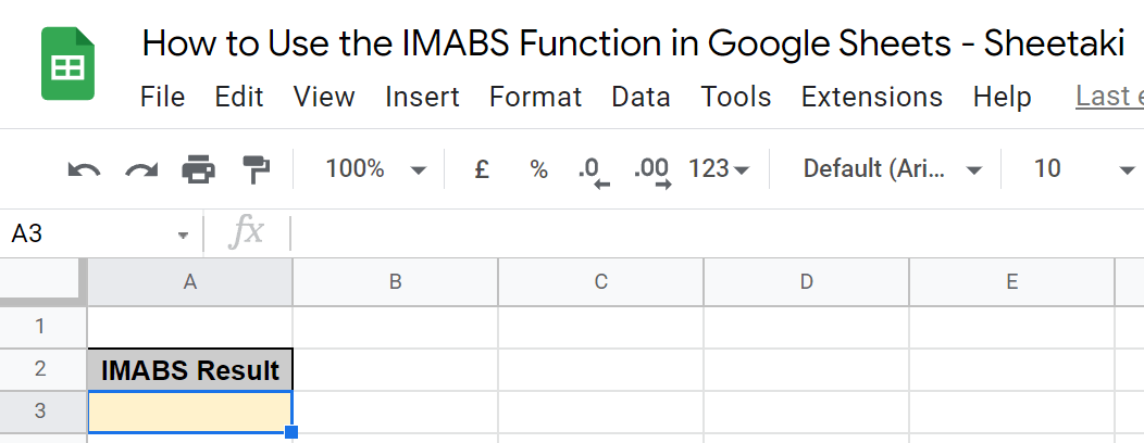
1. First, select the cell where you wish to put the result of your IMABS function. In this case, that’s A3.
2. Next, enter the equal sign ‘=’ to begin the function. Then, follow it with the name of the function, which is ‘IMABS’ in uppercase or lowercase.
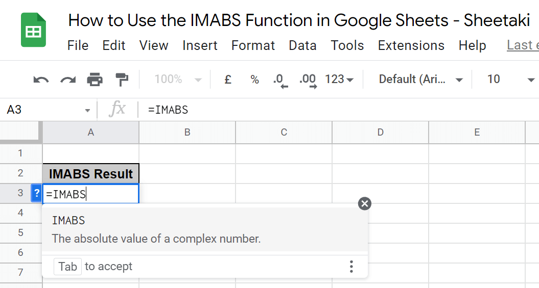
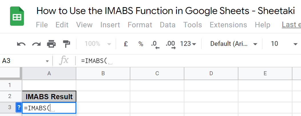
3. Now, either select the IMABS option in the pop-out, hit Tab on your keyboard, or enter an open parenthesis ‘(’ to enable the function.
4. Proceed to enter the complex number, simple number, or cell number that serves as your inumber. Remember to enclose any number with an imaginary part in quotation marks. In this case, we type down “9-3i”.

5. Then, simply enter a close parenthesis ‘)’ and hit Enter on your keyboard.

That’s it! You’ve just learned how to use the IMABS function in Google Sheets.
Frequently Asked Questions
Can Google Sheets use imaginary numbers?
Yes, Google Sheets can use imaginary numbers like how we did so in the IMABS function. It’s symbolized by either i and j. Written in the right format under a function, it should also work under a COMPLEX function and an IMAGINARY Function.
What is a COMPLEX function?
As mentioned, a COMPLEX function can serve as an inumber in an IMABS function since it returns a complex number. It’s formatted as follows: =COMPLEX(real_part,imaginary_part). For example, =COMPLEX(1,2).
Hopefully, this how-to guide has helped you use the IMABS function in Google Sheets properly. Make sure to subscribe and check out the other Google Sheets functions available to learn how to get the most out of Google Sheets. Post your questions in the comment section down below, and our team will help you out!