How to Use IMSINH Function in Google Sheets

This guide will explain how to use the IMSINH function in Google Sheets.

Complex numbers are formed by adding a real number and an imaginary number. A complex number’s real and imaginary parts define an ordered pair that acts as coordinates in a two-dimensional complex plane.

We often need trigonometric functions when working with complex numbers. If we need to find the hyperbolic sine of a complex number in Google Sheets, we can use the built-in IMSINH function.

In this guide, we will cover each step you need to start using the IMSINH function to calculate the hyperbolic sine of a complex number.

The Anatomy of the IMSINH Function

The syntax of the IMSINH function is as follows:

=IMSINH(number)

Let’s look at each argument to understand how to use the IMSINH function.

• number refers to the complex number you want to find the hyperbolic sine of.
• The number argument can either be a COMPLEX function result, a real number, or a string in the format “x+yi” where x and y are valid numbers. The IMSINH number can accept any real number since these values are equivalent to a complex number where the imaginary coefficient is zero.
• The function will return an error if the number argument is not a valid complex number. 
• If you would like to find the sine of a complex number, you should use the IMSIN function instead.

The Anatomy of the COMPLEX Function

The syntax of the COMPLEX function is as follows:

=COMPLEX(real_part, imaginary_part, [suffix])

Let’s look at each argument to understand how to use the COMPLEX function.

• real_part refers to the real coefficient of the complex number.
• imaginary_part refers to the imaginary coefficient of the complex number
• suffix is an optional argument where the user can indicate the suffix to use for the imaginary coefficient. By default, the value for this argument is “i”.

A Real Example of Using the IMSINH Function

Let’s look at a few simple examples where we’ll need to use the IMSINH function in Google Sheets.

Using a cell reference

We can use the IMSINH function to find the hyperbolic sine given a cell reference as input.

Suppose we have a complex number in cell A2. We can determine the sine using the following formula:

=IMSINH(A2)

In the example above, the IMSINH function shows that the hyperbolic sine of the complex number 3+2i is -4.16890695996656+9.15449914691143i.

Using the COMPLEX Function

If you are given just the coefficients of a complex number, we’ll need to use the COMPLEX function to generate a valid complex number for IMSINH. For example, the formula COMPLEX(3,5) returns the complex number 3+5i.

In the example above, we have a table with the coefficients of our complex numbers’ real and imaginary parts. 

We can use the following formula to get the hyperbolic sine given the two coefficients:

=IMSINH(COMPLEX(A2,B2))

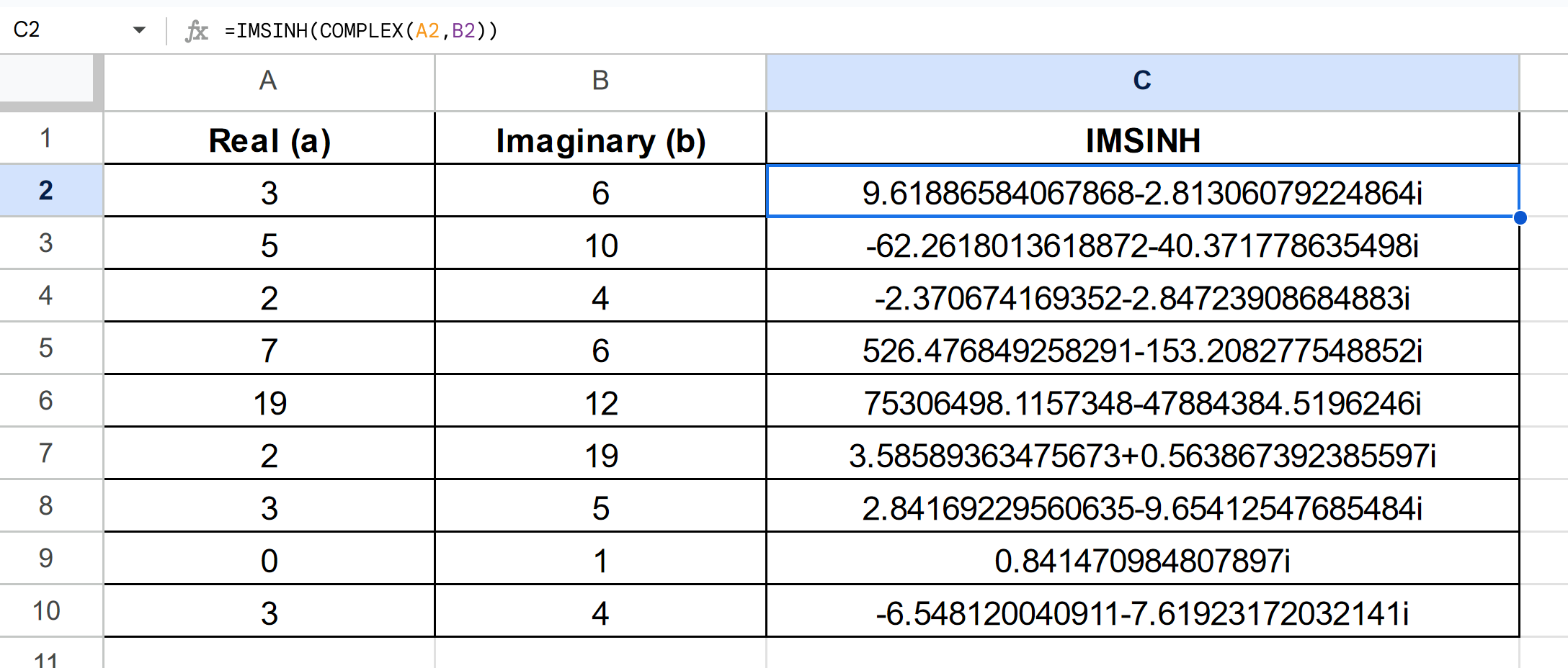
Using this formula, we were able to find the hyperbolic sine values given a set of real and imaginary coefficients.

Click on the link below to create your own copy of our examples.

Head to the next section to read our step-by-step tutorial on how to use the IMSINH function.

How to Use the IMSINH Function in Google Sheets

1. Select the cell where you want to use the IMSINH function.
   
2. Type the IMSINH function and specify a complex number as the sole argument. You may write down a number in the form “a+bi” or a cell reference to another cell with a valid complex number in that form.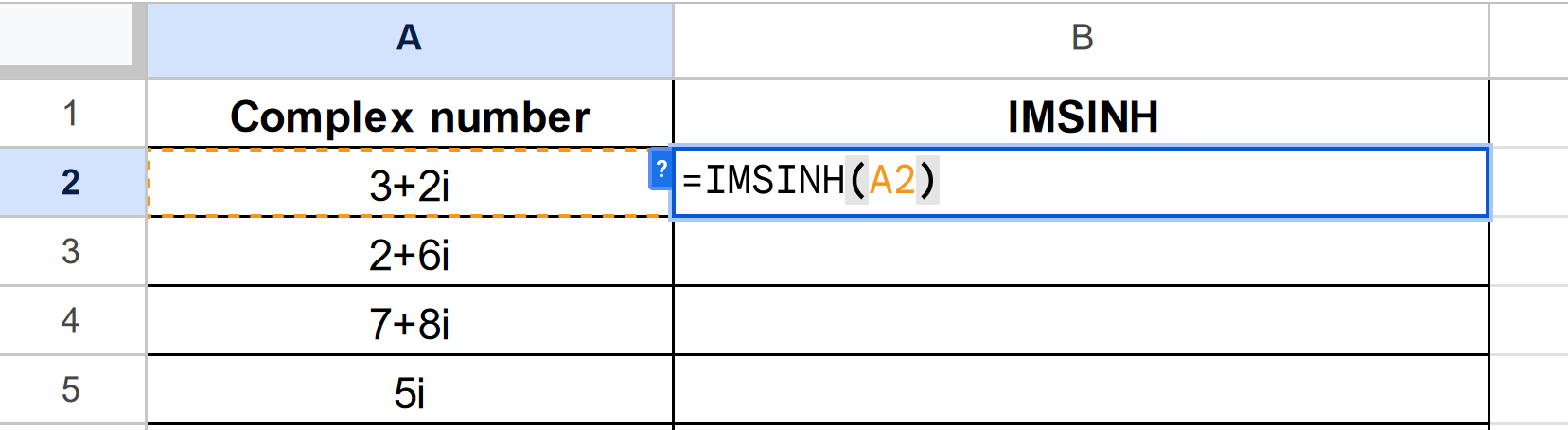
   In this example, we’ll use the formula IMSINH(A2) to find the hyperbolic sine value of the complex number 3+2i.
   
3. Hit the Enter key to evaluate the IMSINH function.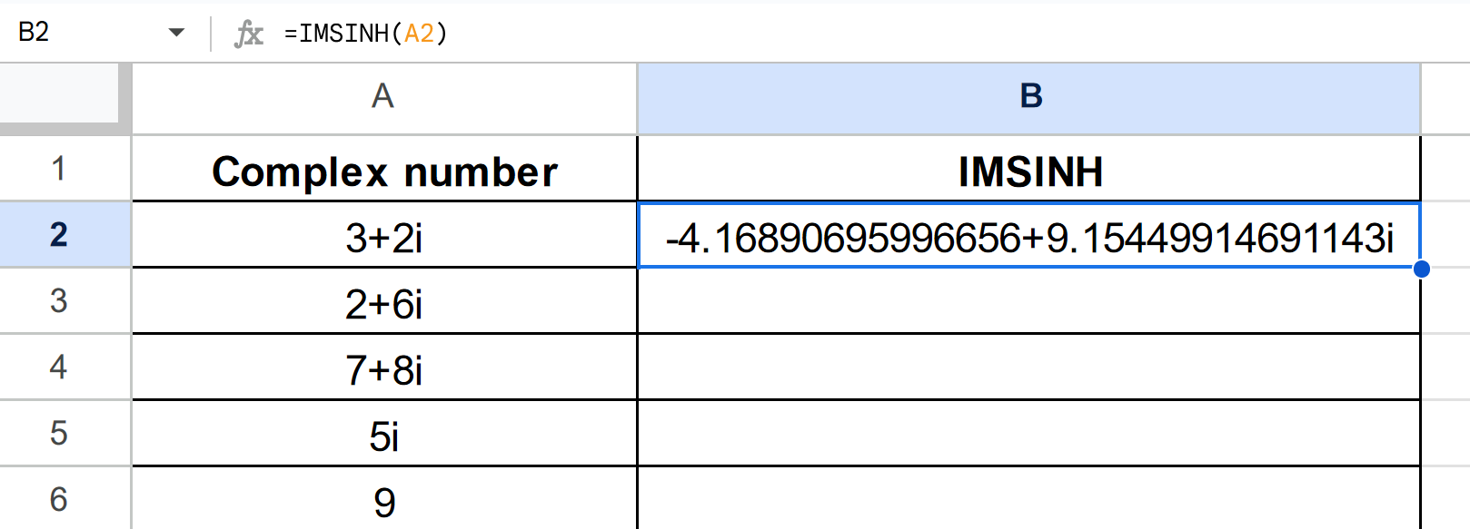
   
4. You can use the AutoFill feature to find the hyperbolic sine of the remaining complex numbers in the table.
   
5. We can use the COMPLEX number to convert the coefficients of our complex number into a valid complex number first.
   In the table above, we’ll use the formula IMSINH(COMPLEX(A2,B2)) to find the hyperbolic sine of a complex number with a real part of 3 and an imaginary part of 6.

These are all the steps you need to know to start using the IMSINH function in Google Sheets.

FAQs

1. Why is my IMSINH function returning an error?
   The IMSINH function may output an error if the complex number you’re using as an argument is not in the proper format “a+bi”. If your complex number is missing the imaginary unit suffix, your function may also result in an error.
   
2. What is the difference between IMSINH and IMSIN function?
   The IMSINH function finds the hyperbolic sine of a complex number, while the IMSIN function calculates the sine of a complex number.

To learn more about using trigonometric functions on complex numbers, you can read our post on how to find the cosine of a complex number in Google Sheets.

That’s all for this guide! Don’t miss out on our library of spreadsheet resources, tips, and tricks!